INTRODUCTION

Airport fog is a longstanding problem.  According to the article at the following link every hour's delay can cost a busy airport $200,000.  Therefore, it is important to identify a method for predicting when the ceiling will lift sufficiently to allow commercial landings.  Ceilometers monitor progress of the cloud base altitude rise once the evaporation phase at the bottom of the fog layer has started, but this is not an adequate solution to the forecast problem because the ceilometer cannot be used to predict when evaporation will begin.  Multiple regression models that use surface properties as input are limited in two ways: 1) the inputs are restricted to surface conditions whereas the process that initiates and drives evaporation in the lowest 200 feet are distributed over that altitude region, and 2) the prediction algorithm, if one is developed for an airport, cannot be transported to other airports with an expectation that it will work as well due to the importance of "local effects."

Intuitively, one should expect that a remote sensing system will be needed to provide the measurement of conditions that are linked to the evaporation process.  The most relevant properties of the lowermost 200 feet, the locusof the burn-off prediction goal, are air temperature and liquid water content.  Each of these properties can be profiled by an appropriate microwave radiometer system.  The rest of this web page explores how such a system might work.

HARDWARE

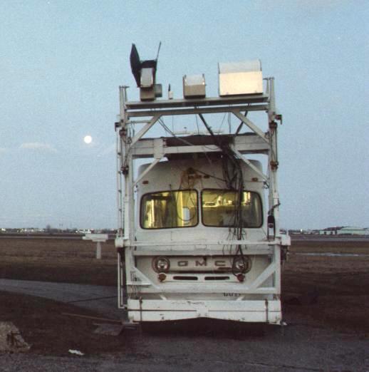
JPL has built and operated many water vapor radiometers and temperature profilers.  Figure 1 is a picture of the MARS system (Microwave Atmospheric Remote Sensor), which was used between 1980 and 1985.  Although it was housed in a large van for several field deployments, it would fit in a smaller van.  The three microwave sensor units on the elevated platform could be combined into one unit, as has been done for later field deployments.  The MARS system will be described because it was used for the measurements to be shown on this web page, which illustrates sensing capabilities relevant to the airport fog burn-off problem.

...

Figure 1.  Microwave Atmospheric Remote Senor system, MARS, which was used on many field deployments during the early 1980s.  All data on this web page were made by MARS.

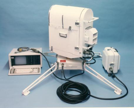
Figure 2.  More compact system designed and built for the Army Atmospheric Sciences Laboratory (White Sands, NM) in 1988, and has essentially the same capability as the MARS van system in Fig. 1. It weighs 169 pounds, can be transported in a car trunk, and includes 4 radiometers that permit temperature profiling, water vapor and liquid water retrievals.

MARS consists of microwave radiometers (passive systems, not involving radar) operating at 22 GHz (mostly influenced by water vapor along the line of sight), 31 GHz (mostly influence by liquid water droplets), 54.0, 55.3 and 57.5 GHz (mostly influenced by the temperature of oxygen molecules at close distances along the line of sight).  The radiometers have small horn antennas that scan an elevation angle range that extends from approximately one horizon, through zenith, to approximately the opposite horizon.  All observations and data analysis are completed in 2-minute cycles.  The next figure shows a sample profile of atmospheric properties derived from a 2-minute data cycle.

The "White Sands" radiometer system operates at 51.07, 53.88, 55.29 and 57.45 GHz, and it measures sky brightness temperature at 5 elevation angles.  The low frequency channel allows useful retrievals to be made of water vapor burden and liquid water burden.  Simulations before delivery indicate the following capability:  T(z) RMS accuracy of <1.0 K from 100 feet to 3000 feet, 1.8 K at 10,000 feet, etc; water vapor burden accuracy of 0.2 cm when clear and 0.7 cm when cloudy; liquid water burden accuracy of 40 microns, average for all sky conditions.  Preliminary measurments made during delivery showed agreement with the predicted T(z) performance, and feedback from the Army also indicates that predicted performance was achieved.  We believe instruments of similar design, such as the Radiometrics systems (whcih are based on the JPL designs), would perform as well if not better than the MARS system.  Therefore, all data shown on this web page should be achievable with a portable radiometer system like the one in Fig. 2.

REAL-TIME OBSERVATIONS AND RETRIEVALS

The following figure illustrates the atmospheric properties that a MARS system is able to determine.

Figure 3.  Example of MARS system retrieved properties.

This data was taken during variable cloud cover conditions, and the cloud properties in the text box summarize statistics for the previous 5 minutes.  From the temperature profile and IR brightness temperature a cloud base altitude was derived; from the temperature profile the inversion base altitude was used to establish the cloud top altitude; and using the thickness of the cloud layer and the liquid burden a LWC (liquid water concentration) was determined.  The dotted trace is temperature from a nearby radiosonde (RAOB), which shows excellent agreement with the MARS-derived temperature profile.  All data except the RAOB profile were produced in real-time by MARS.

The next figure is another presentation of similar data for a time of moderate icing conditions (during the same deployment).

Figure 4.  Three panels showing the same retrieved data at different altitude resolutions. The top panel is for surface to 22,000 feet, the middle panel is for surface to 7300 feet, and the bottom panel is for surface to 2200 feet.   A centigrade scale is shown along the bottom.  The "O" sumbol is MARS-generated air temperature, and the ":" symbol is RAOB measured air temperature.  This particular plot was produced after the ROAB data was available, but a version without the ":" symbols was produced in real-time. A pattern of blanks denote a "dry adiabatic lapse rate line" fixed to the surface temperature.  The presence of cloud liquid water is represented by the "/" symbols.  The upper-right box of text information gives OAT (outside air temperature"), VAP (water vapor burden), LIQ (liquid water burden), IR (8-14 micron infrared sky brightenss temperature), and LWC (liquid water concentration, averaged for the cloud layer).  The lower-left text information box gives aviation icing related information, which was the principal product desired for this field deployment (to the Buffalo Airport).  ICING EXPOSURE is the altitude-integral of icing hazard (defined elsewhere, and scaled to produce values between 0 and 10), CLD TOPS (cloud taop altitude, feet above surface), ICING PK (altitude of maximum icing hazard, in feet), ICING BS (lowest altitude where icing is poredicted to be present, in feet), and CLD BS (ceiling altitude, AGL, in feet).

The data in Fig. 4 was obtained in 1983, which accounts for the "primitive" nature of the display.  Nevertheless, it illustrates what is possible using passive microwave radiometers, supplemented by a cheap IR radiometer.  This display was output to a serial port which was connected to a modem whioch could be dialed-up from anywhere and if the user had the appropriate display connected to his modem the very same display as shown in this figure would be presented.  This capability was successfully used dueing the deployment.

Notice that cloud base and cloud top altitudes are retrieved.  Further, a profile of liquid water content, LWC, are also retrieved.  The retrieval of LWC(z) makes use of the constraint that the integral of LSC with altitude, over a fixed altitude region, is a measured quantity.  A slightly more sophisticated retrieval procedure (Bayesian method) could be employed that makes use of the fact that when a stratus cloud forms water is repartitioned from the vapor phase to the liquid phase, and that the sum of the two forms of water should be approximately constant throughout the boundary layer.  This, and other retrieval sophistications, are currently unexplored future improvements.

How well does the temperature profile compare with radiosondes?

Figure 5.  Examples of two arbitrarily selected MARS comparisons with RAOBs: the coldest and warmest conditions.  This data is from the same Buffalo Airport deployment from which the previous figure was taken.

A thorough analysis of MARS T(z) accuracy was made for the month-long Buffalo deployment, shown in the next figure.

Figure 6.  Summary of a month's worth of comparisons of MARS-generated T(z) with RAOBs, using 28 MARS/RAOB comparisons (13 of which were cloudy). The left most traces are "predicted" performance (dashed) and measured performance (open circles). The right-most traces are inherent variability based on an archive of data from the same site during prior years (dotted) and variability that actually occurred during the observing period (solid circles with heavy trace).

As a "rule of thumb" the MARS temperatures exhibit a 1.0 K accuracy from ground level to 2.0 km, and above 10,000 feet there is essentially no improvement inusing MARS T(z) instead of an archive average.

A 10-month deployment to Denver's old Stapleton Airport in 1985/86 was used to further assess T(z) accuracy for MARS running in an unattended mode.  The accuracy profile for these hundreds of MARS/RAOB comparisons exhibits slightly better performacne than shown in Fig. 4, namely, 1.0 K from surface to 2000 feet RMS = 1.0 K, at 10,000 feet RMS = 2.0 K, at 20,000 feet RMS = 3.0 K.

STRATUS BURN-OFF EXAMPLES

The following examples illustrate occasions when a stratus cloud did NOT burn-off, and two cases when it did.

Figure 7.  Liquid water burden in stratus cloud versus time (continuous trace) and water vapor burden versus time (dots).  A "mist" precipitation occurred for almost an hour. At the top of the figure are notations for surface temperature, cloud base altitude and liquid water concentration, LWC, averaged over the cloud layer.

The integrated liquid content of this startus cloud (continuous trace) did NOT burn-off.  At sunrise the liquid burden was about 400 microns, and at noon it was still about 300 microns.  Based on this "behavior" it would have been easy to predict, for example, that "burn-off during the next 2 hours" was NOT going to occur.  The fact that such a "running prediction" could have been made will be made more clear by the next two cases, when burn-off DID occur.

The cloud layer average LWC is derived by simply dividing the integrated liquid burden by the cloud layer thickness.  Since LWC is expected to rise approximately linearly from zero at cloud base to a maximum value at cloud top, it is possible to estimate LWC at cloud top by doubling the layer average LWC.  Thus, LWC at cloud top was approximately 1.6 [g/m3] in the morning, rose to 2.0 [g/m3] at 10 AM, then slowly returned to the morning values in the afternoon.  The absence of a downward trend in LWC further supports the case that this data could have been used to issue a "NO burn-off in progress" advisory throughout the day.

Temperature profile data may have been taken during this field experiment, but it was not analyzed (since the sponsor did not need that observable set).

Figure 8.  Same labelling as for the previous figure, bu for data of the next day, when stratus burn-off occurred shortly after 3 PM.

During the next day of this deployment a burn-off did occur.  It began at 11 AM, and continued at a constant rate until 3:20 PM, when the liquid burden was under 100 microns.  100 microns is a condition for which shadows are barely visible, and for which it can be said that the burn-off was essentially complete.  Notice that the vapor burden seems "unaffected" by the evaporation of water from the liquid to vapor state.  This is because the water in a liquid phase had a burden of only 500 microns, or 0.05 cm, which is small compared to a total of about 2 cm of vapor burden.  If it can be assumed that a burn-off process will continue at a uniform rate if it has been sustained for at least 2 hours, then at 1:00 PM we could have predicted a burn-off (to 100 microns) of 3:50 PM.  Such a prediction of burn-off in 2.8 hours would have been quite accurate, since burn-off actually occurred at 3:30 PM, or 2.5 hours after the prediction.  At 2:00 PM a prediction would have been made that burn-off to 100 microns would be achieved at 3:40 PM, or in 1.7 hours.  Again, such a prediction would have been quite accurate, since it actually was achieved in 1.5 hours.  Also important to note is that this data could have been used to make "burn-off not imminent" advisories for all times prior to 11 AM.

The layer averaged LWC did not change much during the burn-off process.  Rather, the layer thickness decreased, with the cloud base rising against a constant cloud top altitude, and the liquid burden decreased at a slightly faster rate than the reciprocal of the cloud layer thickness.  As late as 2:30 PM the cloud layer average LWC was only slightly less than its value at 10 AM (0.6 versus 0.7 [g/m3]).  Thus, LWC is not a useful property for predicting burn-off time.

Figure 9.  Stratus cloud burn-off documented at Ontario Airport (in southern California).  Observations began after the burn-off process began, but this data nevertheless shows the well-behaved nature of burn-off until the late stages, when increased convection caused a clumpiness of the overhead cloud liquid content.

The May 21 Ontario Airport burn-off event (Fig. 9) was "slower" than the June 22 Eaton Canyon event (Fig. 8), in the sense that the burn-off rates were 40 microns per hour and 100 microns per hour.

MODEL CONSIDERATIONS

Airport fog along the Western US coast is due to the movement of marine layer air underneath an overlying continental air mass.  The marine layer has a thickness at the California coast that is typically 2000 to 3000 feet.  The water mixing ratio is approximately constant throughout this layer.  The marine layer is overlain by a strong temperature inversion feature, amounting to several degrees K over a 1 or 2 km thick inversion layer.

The key to understanding the evolution of stratus clouds, their formation at night and dissipation during daylight, has to do with the way cloud water drops interact with photons of visible and infrared wavelengths.  Sunlight, consisting mostly of visible wavelength photons, are scattered but not absorbed.  Thermal radiation, consisting of mostly infrarred wavelengths, are absorbed.  This key difference in response to visible and IR photons can account for the major behavior of stratus clouds.  A second physical process to keep in mind for understanding stratus evolution is that water vapor increases the emissivity of an air parcel, but it has little effect upon sunlight.

I will illustrate the iplications of these two physical principles by presenting a temperature profile sequence throughout a stratus episode of one day, using an "intuitive model" to determine the temperature field. The model is "qualitative," not "quantiative," so don't take seriously the exact temperature numbers in the following two figures.

Let us begin with a temperature profile that existed at Vandenberg Air Force Base on June 2, 2000.

Figure  10.  Sequence of hypothetical model of temperature profiles during stratus formation. The marine layer goes from ground level to 500 meters altitude, and throughout this region the dew point is 13.0 C.  Stratus clouds form where the T(z) is colder than the "Dew Point" trace.  Consequently, in this sequence it forms at the top of the marine layer and grows downward.  At 2 AM the stratus cloud extends from 70 meters to the top of the marine layer.  Before sunrise the fog extends throughout the marine layer, from ground level to 500 meters.

The temperature field for this figure is consistent with the measured temperature profile at Vandenberg Air Force Base on June 2, 2000, at the 4 PM sounding.  Stratus conditions are known to have existed in the morning hours following this sounding.  First, notice the is a large synoptic scale compression of downward moving air at this latitude, causing the extensive inversion layer from 500 meters to 1000 meters.  At the late afternoon hours there were no clouds, and the surface is heated enough to produce a super-adiabatic layer below 100 meters.

After sunset the surface has cooled by a large amount due to the ground being a more effective radiator of heat to space than the air.  The dry layer above 500 meters doesn't cool much because it is dry, and lacks emissivity caused by water vapor's absorption spectrum in the IR. However, within the marine layer, which is humid, the air cools at a more rapid rate.  Stratus begins to form when the temperature profile becomes colder than the dew point temperature, and this happens first at the top of the marine layer, at 500 meters altitude, starting at 6:30 PM.  Because water vapor is condensing to liquid water, it releases heat and the cooling rate decreases where stratus is forming.  Hence, initially, the air below the stratus layer cools faster than the air within the stratus.  In addition, the stratus cloud water droplets are able to intercept and absorb thermal radiation from the underlying air, which further retards their radiative cooling rate.  After stratus formation the rate of surface cooling is reduced due to the stratus cloud's absorption of  ground-generated thermal IR radiation and re-radiation back to the ground (prior to which cold space was not radiating significant amounts to the ground).  By 3 AM the stratus cloud extends throughout the entire marine layer in this depiction.

The following figure is meant to represent the sequence of temperature profiles using the same intuitive model for the dissipation process after the sun rises.

Figure  11.  Sequence of hypothetical temperature profiles during stratus burn-off.  According to these profiles the fog begins to burn-off at ground level at 8 AM and the last remnant of stratus is at the top of the boundary layer, which completes its evaporation at 2 PM.

After the sun rises solar energy is reflected and scattered by the stratus cloud droplets, but little of it is absorbed by them.  Most of the sunlight reaching the surface is absorbed because the ground has a low albedo at visible wavelengths.  The heat absorbed by the ground heats the nearby layer of air.  This gradually creates an adiabatic lapse rate layer just above the ground, which initiates convection, and heat is thus exchanged with neighboring layers.  The burn-off thus starts at ground level and raises the stratus ceiling.  In this example the burn-off begins at about 8 AM.  Burn-off is complete by 2 PM.

Notice that the LWC at the top of the stratus is essentially unchanged during most of the burn-off process.  This is consistent with the measurements of Fig. 8, where the LWC averaged throughout the stratus layer was essentially constant during most of the burn-off phase.

This example of temperature profiles during the formation and dissipation phases of a stratus cloud is meant to convey the complicated nature of the stratus problem.  The temperature profile structures will not be neat, straight lines.  Nevertheless, the temperature profiles will reflect where heat is being absorbed or lost, and temperature profiles should be a key diagnostic of the entire stratus evolution process.

SPECIFIC AIRPORT FOG INSTRUMENTATION SUGGESTION

A first reaction to the temperature field behaviors illustrated in Fig. 11 is to wish for an instrument system that can monitor the temperature field at the lowest altitudes.  However, consider the fact that as energy is being absorbed by this lowest altitude layer the main effect is to reduce LWC, while only slightly increasing temperature.  Thus, the most desireable instrument system would be one that measures LWC somewhere within the lowest 200 feet.

Fortunately, it is possible to build an instrument that both measures LWC profiles at low altitudes, but also measures temperature profiles in the same region.  It is a microwave radiometer similar to the many previously-built Microwave Temperature Profilers.  I will refer to it as the "Fog Microwave Radiometer," or FMR.

    Airport Fog Microwave Radiomter

        Channel 1 = 50 GHz
        Channel 2 = 56 GHz
        Channel 3 = 64 GHz
        Channel 4 = 61 GHz
        Channel 5 = IR (8-14 microns)

This radiometer system should scan through a elevation angle arc extending from near the horizon (such as 5 degrees) at one azimuth, and going though zenith to the opposite azimuth near the horizon.  By this means it will be possible to minimize confounding effects of horizontal inhomogenieities of cloud LWC.  The rationale for such a selection of frequencies rests upon the different spectrae for oxygen and liquid water drops, as shown in the next figure.

Figure 12.  Microwave spectrum for a typical sea level atmosphere without stratus clouds (1000 mb, 10 [g/m3] water vapor) and three stratus cloud liquid water concentrations, LWC.

The choice of working with frequencies that straddle the peak of the oxygen lines (near 60 GHz) allows for the separation of the effects of cloud liquid water from an unknown temperature profile, and has been suggested by Westwater (19??), and also by Mahoney (2000).  The technology for building such a radiometer is well-understood, and is a minor variant of the many Microwave Temperature Radiometers that JPL has built, and that Radiometrics Inc. now builds commercially.

Inclusion of an IR radiometer enables cloud ceiling to be determined, as the IR brightness temperature will match the microwave-derived temperature profile at just one altitude, which will be the ceiling.  This procedure was demonstrated by MARS, and examples of these determinations can be seen in Fig.'s 3 and 4.

The microwave component of the FMR could be the same size as the Army radiometer shown in Fig. 2.  The IR radiometer could be a hand-held (though hard point mounted) "IR gun" (costing $1500), similar to the one used in MARS.

The retrieved products for the FMR would consist of the following:

    1)  T(z) from z = 50 feet to 1000 feet (in heavy fog) or 5000 feet (in the absence of stratus fog)
    2)  LWC(z) from z = 50 feet to 1000 feet (in heavy fog)
    3)  Vapor burden when stratus cloud liquid burden < 1000 microns
    4)  Liquid burden of stratus cloud

These retrieved properties would allow for the monitoring and prediction of stratus formation as well as stratus dissipation.  In other words, closure times as well as re-opening times could be predicted.

THE NEXT STEP

Before proceding with the construction of a proto-type FMR it would be prudent to quantify the stratus formation and dissipation evolution scenarios presented here, based on my "intuitive model."  If the quantitative model confirms the fact that LWC changes faster than T(z) in the lowest 200 feet during burn-off, then a specific FMR instrument design should be formulated.  Next, a simulation of FMR observables with a realistic stratus formation and dissipation scenario should be conducted.  This will verify that the observables ahve the power to monitor changes and predict future states during the critical phases of formation and dissipation.  These paper studies should be conducted in collaboration with a competent meteorologist having experience with stratus models.

JPL has already collaborated with UCLA meteorologists on a stratus formation and dissipation project, involving water vapor radiometers and microwave temperature profilers provided by JPL and stratus model development by UCLA.  The observations were taken at the El Monte airport in 1977, during a 5-day period, with vapor and liquid burden measurements provided by JPL and support measurements provided by UCLA personnel; these data were used to constrain a stratus model developed by a UCLA doctoral student under the direction of Prof M. Wurtele.  A similar dual observational and theoretical collaboration might be appropriate for the development of an optimum FMR.

FOG MICROWAVE RADIOMETER STUDIES

To view a description of a hypothetical Fog Microwave Radiometer, and a simulation of FMR Observables versus time during a fog formation and dissipation process, go to the following link.

Link to an ongoing measurement program to study stratus cloud formation and dissipation conducted from site in Santa Barbara.

References

Mahoney, M. J., 2000, NASA Tech Briefs, Photonics Tech Briefs, May, p. 23a.

Westwater, 19??

This site opened:  January 7, 2001.  Last Update:  May 31, 2001