EXOPLANET TRANSIT OBSERVATION
SYSTEMATIC ERRORS
Bruce L. Gary; Hereford, Arizona; 2007.02.18
This web page is meant for amateur observers of exopanet
transits wishing to reduce systematic errors in order to achieve more
accurate transit depths and mid-transit timings. I will use my
observations to illustrate systematic errors that may be present.
INTRODUCTION
An exoplanet transit observation will typically be 4 to 8 hours long
and during that time several systematic errors may vary in severity in
a way that distorts the shape of the transit light curve. For example,
it is common for pre- and post-transit baselines to differ by 1 or 2
mmag (milli-magnitude). This may not be important if the transit depth
is greater than 30 mmag, but for 10 mmag depths it will be important.
It is therefore important to have observations for long streatches of
pre- and post-transit times in order to assess the magnitude of
systematic errors that will surely pe present at some level. The
purpose of this web page is to identify several sources of systematic
errors that an amateur, such as myself, is likely to be present, and to
suggest ways to minimize them.
Since I will be using real data to illustrate these errors I should
describe my observing systems. I use the plural "systems" because even
with one telescope it will matter whether you are configured Cassegrain
or prime focus, and whether a dew shield is used, or whether a focal
reducer lens is used, and where it's inserted. Every change of
configuration will change the relative importance of the various
systematic error sources. During the past year I have had three
different telescopes, so I can also address some issues related to
telescope design differences - such as meridian flip effects. All of
these telescopes have been 14-inch apertures catadioptics: Celestron
CGE-1400, Meade RCX400 and Meade LX200GPS. Most of my
illustrations will be with the last one. I use a sliding roof
observatory, so wind shaking is important whenever they exceed ~5 mph.
My site is in Southern Arizona, at an altitude of 4660 feet; my
atmospheric extinction values for B, V, R and I bands is typically
0.25, 0.16, 0.13 and 0.058 magnitude per air mass.
Here is a list of systematic error sources, with internal links to their discussion:
1) Air mass correlated errors due to reference stars having different color than target star
2) Defocus drift
3) Photometry aperture too small
4) PSF different near edges where some reference stars are located
5) Thin cirrus
6) Wind shaking telescope and atmospheric waves
7)
Air Mass and Reference Star Color Differences: Example 1
Star color effects will be greatest when observng unfiltered. The
first example illustrates the effect of reference star color on transit
depth using a set of unfiltered images.
The following star field was calibrated using all-sky photometry
techniques that transfer standard Landolt star magnitudes to an unknown
star field.
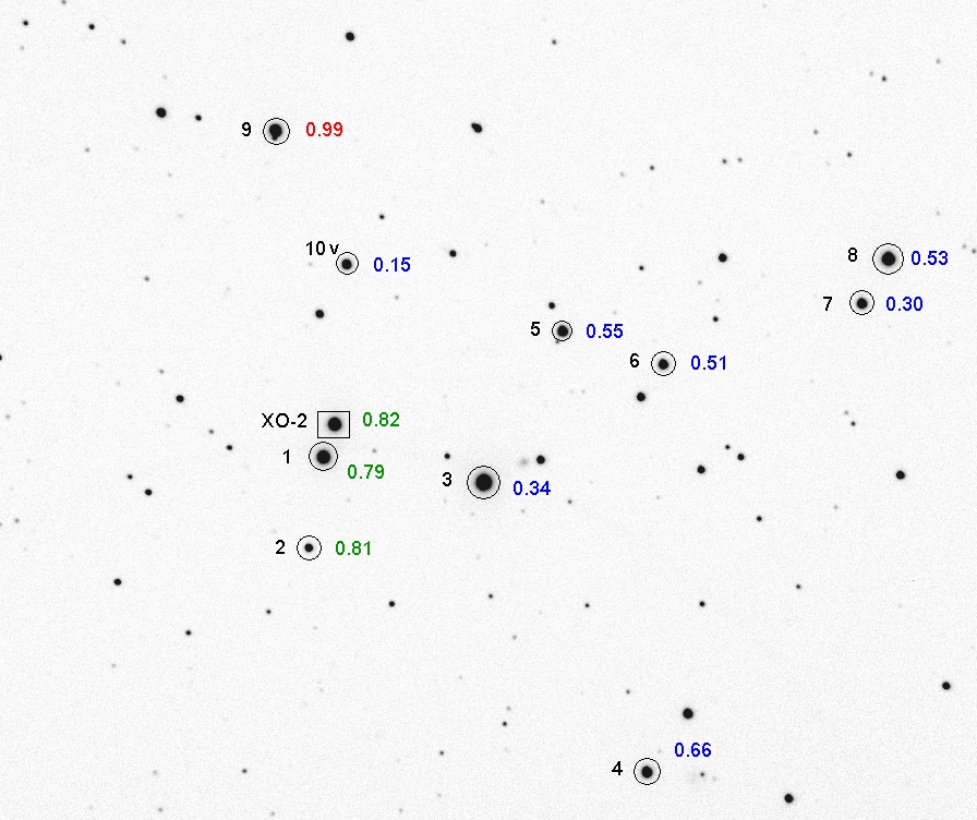
Figure 1. B-V colors of stars near a transiting exoplanet.
Star 1 is the same color as the exoplanet star (both of which are in
orbit around each other, and also are the same brightness). It was used
as a reference star to produce a light curve (LC) that will be adopted
as "true." This choice for reference star also has the merit of being
close to the target star (the exoplanet star) and having the same
brightness as the target star. This LC is the top one in the next
figure.
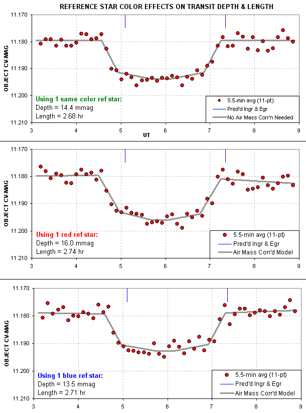
Figure 2. Transit light curves using 3 choices for reference star.
Notice the transit depth differences for the three reference star
choices. Using a red reference star (Star 9) leads to a depth that is
11% too high. using a blue reference star (Star 3) leads to a depth
that is 6% too low. Also note that the time of ingress and egress
depend on which reference star is used. This means that the mid-transit
time depends on reference star color.
Flat field imperfections should be almost non-existent for these LCs
since a SBIG AO-7 image stabilizer kept the star field fixed with
respect to the pixel field to within about 2 pixels (less than the PSF
width). The air mass range was small, as shown in the next figure.
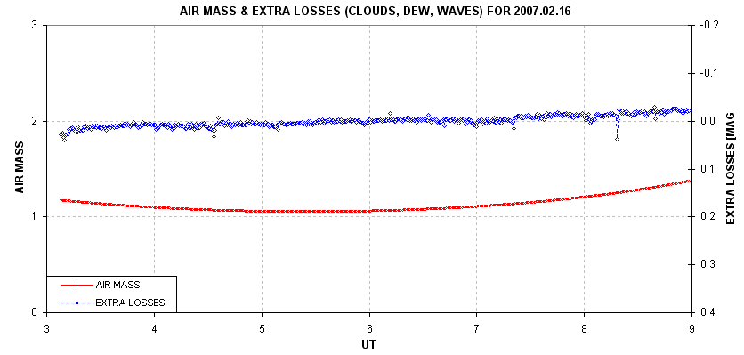
Figure 3. Air mass (red) and extra losses due to clouds and poor seeing (blue) for the observing 2007.02.16 session.
If measureable depth systematic errors are present for this
observing session, with an air mass range of only 1.06 to 1.38, we
should expect that a less favorable observing situation, with a larger
air mass range, would produce larger transit depth effects.
Air Mass and Reference Star Color Differences: Example 2
This section is for R-band observations covering a larger air mass
range. I use it to show that even R-band observations can exhibit
transit depth effects related to air mass. A larger range of air mass
is used in this example, but unfortunately the observing session was
for a "no show" exopanet candidate. Therefore, I'll have to argue what
would have been measured for transit depth based on the baseline
curvatures that are measured. The next figure shows a LC of a normal
star when using a very red star for reference.
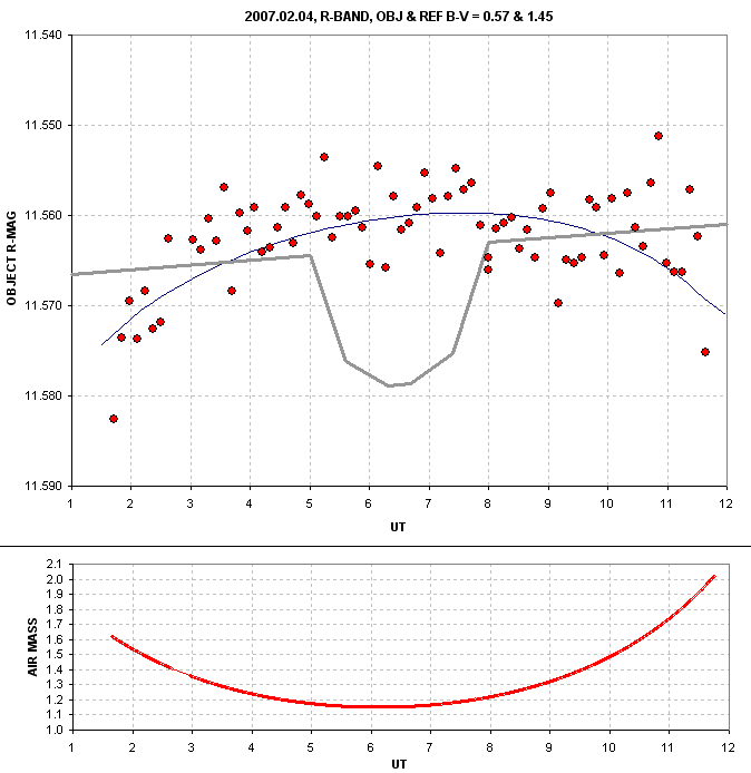
Figure 4. R-band measurements of a star having B-V = 0.57 (normal) while using a reference star having B-V = 1.45 (very red). The thin
blue trace is a model fit using air mass and time as independent
variables; the time component of the model causes the maximum to occur
~1 hour after transit. The grey transit trace is hypothetical, with a 3-hour length and 15 mmag depth and a -0.5 mmag/hour drift.
If a 15 mmag transit had occurred it would have been measured as having
a 11 mmag depth due to the dependence of systmematic error on air mass.
The effect would have been less if the transit had not been centered on
minimum air mass, or if it had been shorter. Also note that if the
transit had occured there would have been insufficient data to be
certain that a baseline curvature was present. The small temporal
effect (0.5 mmag/hour) is easily determined whenever there is
sufficient baseline before and after the transit event.
We'll now try to determine the cause for each baseline departure from flat (curvature and slope).
What could have caused the curved baseline? Note that only one
reference star was used and it was very red (B-V = 1.45, according to
the USNO-A2.0 catalog). A red star will not vary as much with air mass
as a blue star. Since the "object" was bluer than its reference, it
would have faded with air mass at a greater rate, causing it to be
brightest near transit. If this theory is correct then we should be
able to show that using a blue star as reference for a red star the
reverse curvature should be produced. We'll do this with the same set
of images, using two different stars.
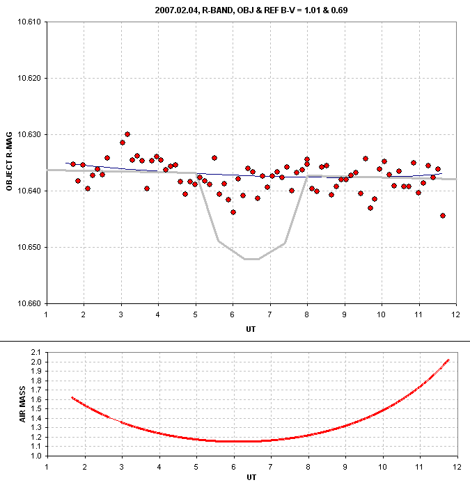
Figure 5. Light curve of a slightly red star (B-V=1.01) using a normal star (B-V=0.69) as a reference.
As expected, the curvature reverses when the colors of the object and
reference are reversed. If a 15 mmag deep transit had occurred its
depth would have been measured as ~14 mmag. In this case the stars had
a small color difference, so the curvature is small, yet it is in the
expected direction. This supports the theory that the color of
reference stars matters when doing high precision light curves.
Let's prove that the curvatures demonstrated can be produced by the
star color differences and air mass range used in the two examples.
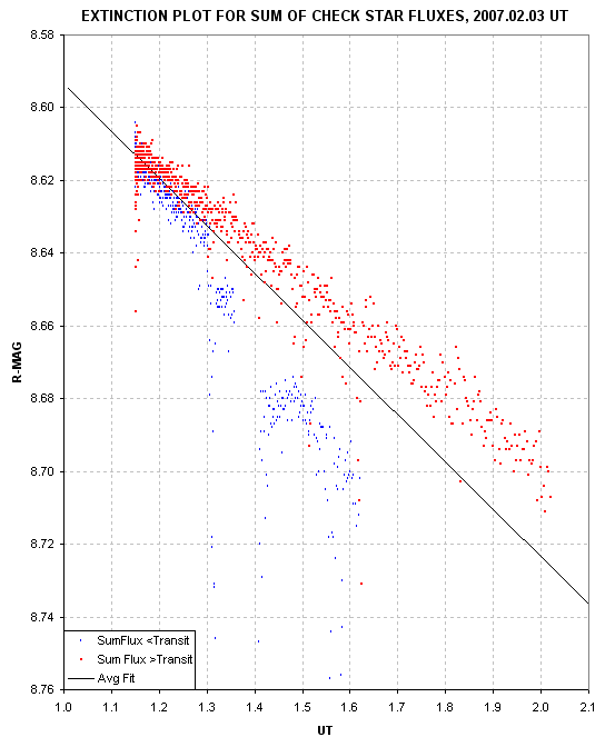
Figure 3. Star flux versus air mass had a steeper slope (zenith extinction) before transit than after transit.
Defocus Drift
I once neglected to "lock the mirror" after establishing a good focus,
and went to sleep while observing a transit candidate. I'm glad this
happened, because the focus drifted and caused an effect that was too
obvious to ignore. The way the problem showed itself was a slow "brightening" of
the target (in relation to several reference stars) near the end of the observing session (while I
slept). This is shown in the next figure.
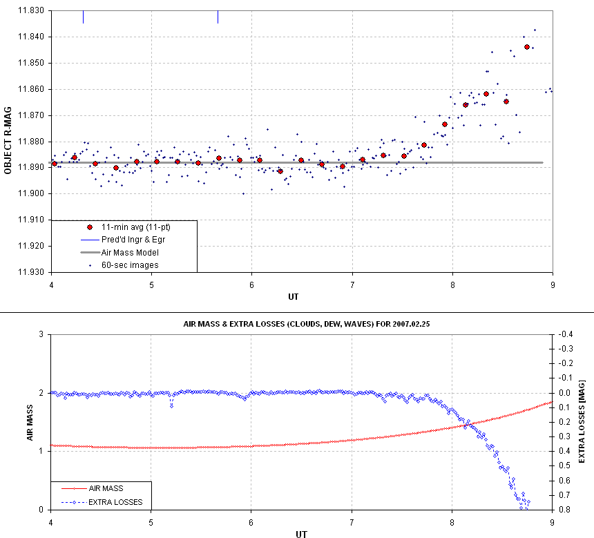
Figure 4. Light curve showing effect of focus drifting away
from "sharp" starting at ~7.2 UT. The lower blue trace shows that the
total flux for all reference stars decreased starting at the same time.
I recall upon awakening, and looking at the image on the monitor, that the focus was bad, but I didn't know what
effect it would have on the LC. When I saw the LC I right away
suspected focus drift had something to do with it. Here's a plot of FWHM for the images used in the above figure.
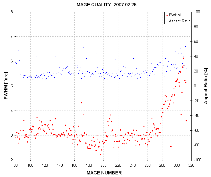
Figure 5. Plot of FWHM ["arc] and "aspect ratio %" (ratio of
largest PSF dimension to smallest, expressed as a percentage) for the
images used to produce the previous figure. Image numbers near 260
correspond to 7.0 UT.
There's clearly a good correlation of when focus degraded and when the
apparent brightness of the target star began to increase (~7.0 UT). But
how can an
unfocused image affect the ratio of star fluxes? To determine this,
consider
how MaxIm DL (and probably other programs as well) establish magnitude
differences from a set of images. I'll use two images from the above
set
to illustrate this.
An image in good focus was chosen from ~7.0 UT and another from ~8.5
UT. They were treated as a 2-image set using the MaxIm DL photometry
tool. The next figure shows the sharp focus image after a few stars
were chosen for differential ensemble photometry.
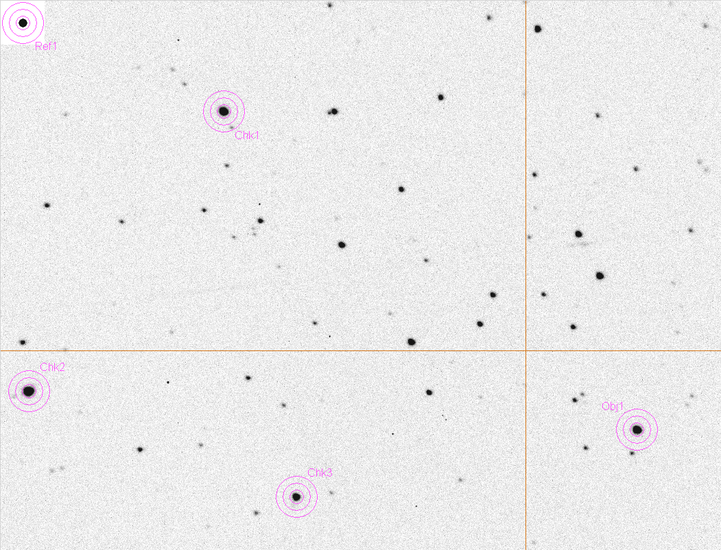
Figure 6. Screen capture of the photometry apertures after
using this image to select an object star, check stars and a reference
star (upper-left corner, my artificail star).
Note that essentially all of each star's flux is contained within the
signal aperture. The next figure is a screen capture of the unfocused
image.
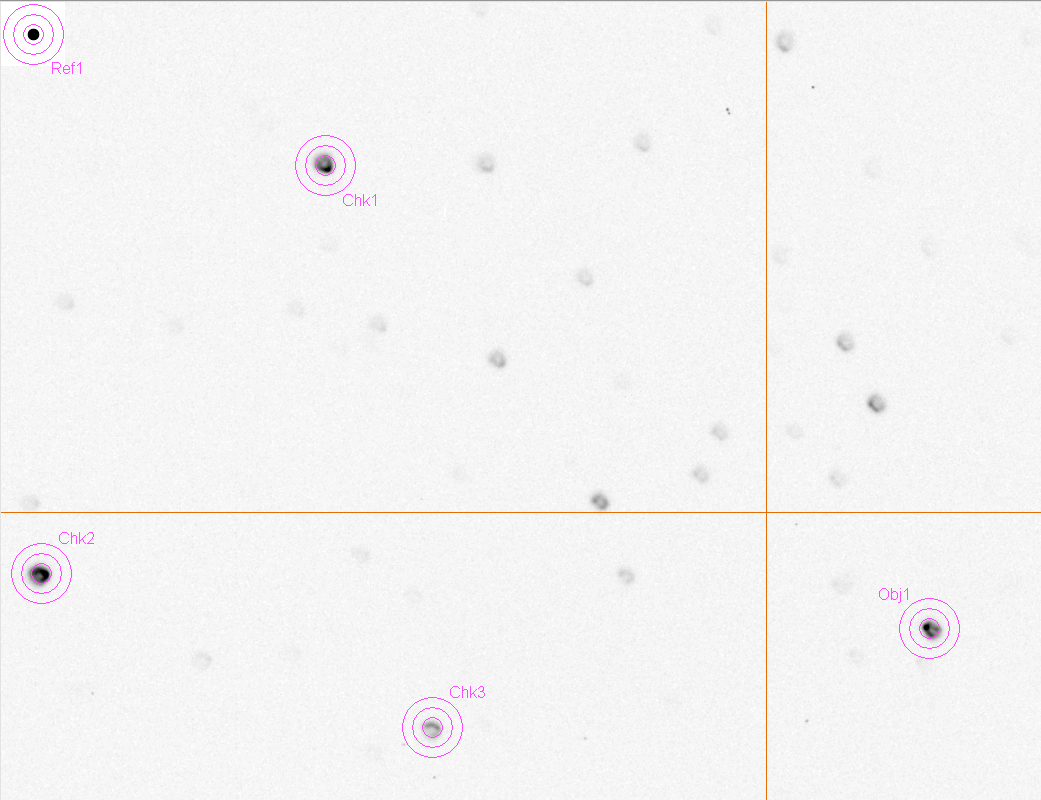
Figure 7. Same photometry apertures (at the same x,y locations as in the previous image) for the defocused image.
Notice that in the defocused image the star flux is spread out in
different directions (away from the center of the image) and also
amonts that are greater the farther the star is from the center. Thus,
stars near the edges have a smaller fraction of their total flux within
the aperture than stars near the center. The ratio of fluxes, and hence
magnitude differences, and affected. The effect on the object's
measured brightness can have either sign, depending on whether the
object or stars used for reference are closer to the center of the
image. Presumably this effect could be
reduced by using a larger signal aperture. The best solution is to use
only sharply-focused images.
Referring back to Fig. 4, and noting the blue trace labeled "Extra
losses [mag]", a decrease of such a trace is usually produced by cirrus
clouds. However, in this case it was produced by a spreading out of the
PSF beyond the signal aperture circle as focus degraded.
____________________________________________________________________
This site opened: February 15,
2007 . Last Update: February 26,
2007