This
"tutorial" is written for those employees
of Rockwell International (especially the Collins Air Transport
Division) who
want a general understanding of how microwave radiometry works, and how
instruments employing this technology can provide information useful to
pilots.
Microwave
radiometer instruments are potentially useful
in the following three areas:
1)
Low
Altitude Wind Shear (LAWS),
2)
Clear Air Turbulence (CAT), and
3)
Flight level selection for fuel savings.
Since
infrared technologies are also potentially useful
for the LAWS and CAT applications, I will occasionally highlight
significant
differences of the two technologies for these two applications.
Measurement
concepts for microwave radiometers are
explained in sufficient detail to enable the reader to compute observed
quantities for simple cases not explicitly treated in the text. This has been done at the risk of boring the
"executive" reader, so I have tried to indicate which sections can be
skipped without losing the "flavor" of what microwaves are good
for. The executive reader is now invited
to scan the next two major sections and then begin reading the
sub-section
"Altitude Temperature Profiles."
THERMAL
RADIATION FUNDAMENTALS
Microwave
photons, like all photons, interact with all
matter, whether the matter is solid, liquid, gaseous or plasma. The term "interaction" means that a
photon can be absorbed by the matter, reflected by it, refracted by it
(after
entry into it). Photons can also be emitted by matter. Emitted
photons are called "thermal
radiation" (therea re a few minor exceptions, such as synchrotron
radiation, masers and lasers, etc., which are called non-thermal
radiation).
The
probability of an interaction of a photon with matter
depends on the wavelength of the photon and the matter in question. There is a maximum rate which a
"simple" material (at uniform temperature throughout) can emit
"thermal" photons per wavelength interval. A
material emitting photons at this maximum
rate (at each wavelength) is said to be a "blackbody."
Blackbodies
emit photons across the wavelength spectrum
with predictable energy output per wavelength interval given by the
famous
Planck Equation. For long wavelengths
the emitted energy is proportional to the temperature of the material. For short wavelengths the emitted energy is
strongly dependent on temperature.
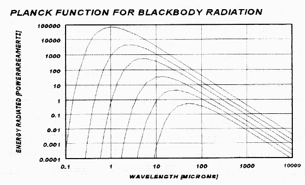
Figure 1. Planck
Equation showing radiation intensity versus wavelength for the
temperatures 100, 200, 400, 1000, 2000, and 5000 K. Power radiated is in relative units.
For objects at everyday temperatures microwaves are "long." For these objects the emitted energy is proportional to temperature, provided the wavelength is much longer than about 4 microns. For most infrared radiometers (8-14 microns, for example) the energy per unit wavelength interval varies in a more complicated way with temperature. At wavelengths shorter than about 4 microns the emitted thermal radiation is so weak that it is easily overwhelmed by even small amounts of reflected sunlight, street lights, etc.
A
microwave radiometer is simply a device whose output is
related in a linear manner to the number of photons emitted by the
material
being "viewed." Since a
doubling of the flux of photons is produced by a doubling of the
physical
temperature (Kelvin temperature) of the material, the radiometer
provides a
simple means for measuring the physical temperature of the material. Since this measurement can be made from a
distance from the object, a microwave radiometer is a remote sensor for
measuring an object's physical temperature.
All
materials absorb photons with some finite probability
per photon. Liquids and solids generally
have properties that vary slowly with wavelength, although some
minerals have
resonance features at specific wavelengths.
Molecules in a gaseous medium that absorb photons may move their
electrons to higher shells (possibly becoming ionized), they may
vibrate more,
or they may rotate faster. All these
changes are "quantized." The
energy quantization for molecular rotation is smaller than for the
other changes. Thus, long wavelength
photons are capable of
changing molecular rotation.
ATMOSPHERIC
ABSORBERS/SCATTERERS
The
following sub-sections survey atmospheric
constituents that either absorb or scatter at frequencies near 60 GHz
and
wavelengths in the 8 to 40 micron region.
The next major section
discusses how to use this absorber/scatterer information to calculate
observed
microwave brightness temperature for hypothetical atmospheres, and how
to do
the reverse - to convert measured brightness temperature to desired
atmospheric
properties. Some readers may want to
merely browse through the following sub-sections and give more
attention to the
next major section.
Oxygen
Oxygen
molecules have quantized rotations corresponding
to the energy carried by microwave photons with wavelengths of
approximately 5
millimeters (frequencies of about 60 GHz).
Several dozen of these quantized states exist within the
frequency
interval 48 to 71 GHz (one exists at 119 GHz).
At sea level the atmospheric pressure is so high that collisions
between
the molecules distort them enough to "smear" the spectrum of
interaction probability versus frequency.
Thus, at sea level the absorption coefficient of oxygen versus
frequency
is a smooth function throughout the 50 to 70 GHz region.
At higher altitudes there is less
"smearing," and the individual resonance absorption lines can be
easily discerned. This is the so-called
resonant absorption spectrum of oxygen in the microwave region (see
Fig. 2).
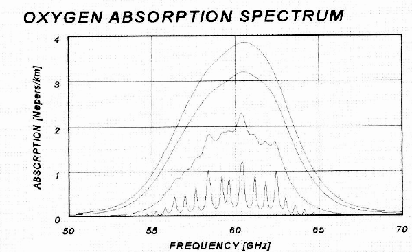
Figure 2. Absorption spectrum of oxygen for altitudes 0, 2, 10 and 20 km.
Absorption
coefficient, Kv,
is given in units of [Nepers/km] in this tutorial.
To convert to [db/km] multiply the
[Nepers/km] value by 4.343. In a medium
where Kv
= 1
[Nepers/km] a photon will have a 1/e = 0.37 probability of being
transmitted
(and a 1 - 1/e = 0.73 probability of being absorbed) after traversing 1
km
within the medium.
Carbon
Dioxide
Carbon
dioxide does not absorb below frequencies of 115
GHz, so it is of no concern to microwave radiometers operating in the
60 GHz
region.
In
the IR there are strong absorption bands, such as at
14 to 16 microns. Since CO2
is a well-mixed atmospheric gas, and since its absorption properties
are known,
it is possible to predict CO2 absorption at all altitudes. This CO2 IR absorbing feature is
similar to the 60 GHz O2 microwave absorbing feature in the
sense
that both wavelength regions can be used for remotely sensing the
temperature
of the atmosphere. However, since some
of the individual lines in the 14 to 16 micron region are very
temperature
sensitive care must be taken in calculating a predicted temperature
sensitivity
that matches the specific IR radiometer's passband.
Water
Vapor
Water vapor has resonant absorption features as well as a non-resonant component. Two significant water vapor resonances occur at 22.2 and 183 GHz. The shape of the total water vapor absorption spectrum for the 10 to 70 GHz region is presented in Figure 3.
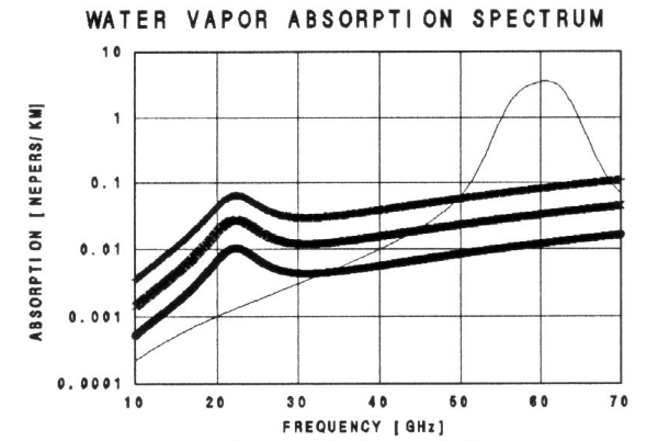
Figure 3. Water
vapor absorption spectrum for typical surface conditions: air
temperature = 15 C, RH = 15, 40 and 95% (1.9, 5.2 and 12.3 [g/m3]). Note absorption spectrum for oxygen.
In
the region 50 to 70 GHz water vapor is less absorbing
than oxygen. Water vapor concentration
decreases rapidly with altitude (since temperature decreases with
altitude and
the saturation vapor pressure decreases with temperature).
The scale height for water vapor is
approximately 2 km, instead of the 8 km for the well-mixed gases
(nitrogen,
oxygen, etc.). Above approximately
10,000 feet it is possible to neglect the effect of water vapor for
radiometers
operating in the oxygen absorption region (50 to 70 GHz).
It is even possible to neglect the effect of
water vapor at low altitudes in the middle of the 60 GHz oxygen
absorption
complex, except under warm and humid conditions.
IR
photons are affected by water vapor if they are close
to water vapor resonance absorptions lines.
The strongest IR absorbing features are at 5 to 8 and 19 to 300
microns.
Cloud
Liquid Water
Liquid
water droplets (ie, all clouds except cold cirrus) can
be important absorbers for
microwave radiometers. They do not have
resonant absorption features, but the non-resonant absorption increases
with
the square of frequency (throughout most of the microwave region). Figure 4 shows the liquid water absorption
spectrum for three cloud water concentrations.
To
illustrate the effect of low altitude clouds on
microwave measurements, consider a stratus cloud that is on the verge
of
drizzling. It will have a liquid burden
of about 700 microns and a thickness of approximately 0.7 km. This corresponds to a Liquid Water Content,
LWC = 1 [gm/m2]. The
absorption coefficient of such a cloud in the 50 to 70 GHz region is
0.5
[Nepers/km]. This is comparable to
levels sea level oxygen absorption values, which are 0.1 to 4
[Nepers/km]. There are some situations in
which it is not
necessary to take this into account (ie,
when measuring lapse rates at flight level), and other situations in
which it is necessary (ie, measuring
horizontal temperature gradients at large distances).
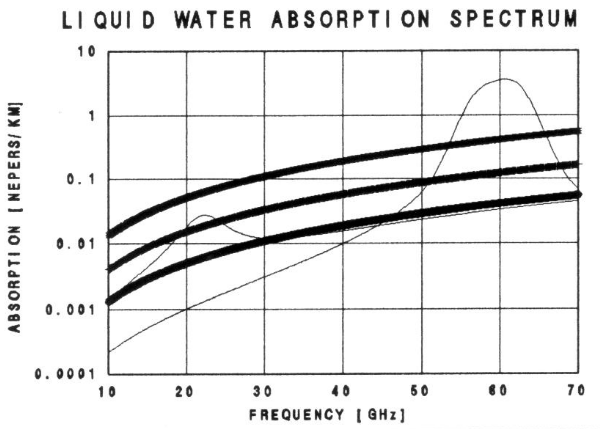
Figure 4. Liquid
water (droplet) absorption spectrum for LWC = 0.1, 0.3 and 1.0 [gm/m3]. Absorption spectrum for oxygen (at sea level)
and water vapor (40% RH at 15 C) are also shown.
For
cumulus clouds, with LWC »
0.1 [gm/m2], Kv
due to liquid water »
0.05
[Nepers/km]. This is small but not
negligible compared with oxygen absorption, and the same comments in
the last
paragraph apply here.
At
cruise flight levels LWC is even lower, and microwave
absorption coefficients are correspondingly lower for a given
temperature. It should be noted that
liquid water's
absorption coefficient increases as temperature decreases.
Kv
increases approximately 28% per 10 K temperature
decrease. Thus, a cloud with LWC »
0.1 [gm/m3] has Kv
»
0.076
[Nepers/km] at -10 C instead of 0.046 [Nepers/km] at +10 C.
Cloud
droplets scatter, but near 60 GHz the scattering is
insignificant compared to absorption.
Infrared photons, due to their shorter wavelength, experience
(Mie)
scattering that is far greater than the low levels of (
Rain
Rain
drops are large enough to cause scattering losses that
can be a few tens of % of the raindrop absorption at
60 GHz for large rain
drops. Nevertheless, absorption is still
the more important effect, and for most situations scattering can be
ignored.
Since
infrared wavelengths are short compared with
raindrop sizes they are scattered at significant levels.
IR radiation is also highly absorbed within
rain. {?? more info needed here ??}
Ice
Absorption
Water
ice is essentially transparent to microwave
photons. I have calculated that a
typical cirrus cloud must be 400 km deep to provide an optical depth of
1 at 60
GHz (ie, Kv
»
0.0025
Nepers/km). This is 2 to 3 orders of
magnitude less than oxygen absorption (at cirrus altitudes).
IR
photons are both scattered and absorbed by ice
crystals, though absorption is usually greater.
Many cirrus clouds are optically thick at IR wavelengths, which
can lead
to strong radiative cooling at their tops (due to loss of energy by
radiation
of IR photons to cold space) and strong radiative warming at their
bottoms (due
to absorption of earth surface IR thermal radiation).
IR remote sensing is probably hopeless while
flying through cirrus clouds!
Aerosols
Non-water
aerosols consist of dust and smog (at low
altitudes) and condensation nuclei, polar stratospheric clouds and
volcanic ash
(at high altitudes). All of these
aerosol types produce negligible absorption and scattering of
microwaves.
For
example, a dust storm which obscures visible light at
the rate of "one optical depth per 500 meters," which would cause an
e-folding loss of visual signal every 500 meters, exhibits an
absorption at 60
GHz of 0.3 % per 500 meters (I assume 100 micron diameter dust
particles). This is negligible,
considering that oxygen
absorption is 2 to 3 orders of magnitude greater. By
a similar argument it can be shown that
high altitude condensation nuclei produce negligible absorption at 60
GHz.
IR
wavelengths are much smaller than the assumed dust
grain size, so pure geometrical considerations show that the scattering
loss
will be 1 Neper per 500 meters, or 2 Nepers/km.
Absorption losses will also occur.
Therefore, interpretation of IR measurements will be ambiguous
in dust
storms (similar to the one in this example).
Smog
does not absorb appreciably in the microwave
region. From the perspective of the smog
remote sensing community it would be good if smog did
have absorption features, but none exist close to 60 GHz.
IR
probably has smog absorption resonance features in the
absorption spectrum (ie, NOx),
but I do not know if smog absorbers are important for the endeavor of
remotely
sensing air temperature in the 15 micron region. {?? more info needed
here ??}
Condensation
nuclei (CN) at high altitudes are much
smaller than IR wavelengths, so scattering will be comparable to
molecular
|
Table I Which Constituents Are Important? Constituent 60
GHz IR Oxygen Yes/No Yes/No CO2
No
Yes/No Water
Vap/surf Yes/No Yes/No Water
Vap/alt No
Yes/No Liquid
Water Yes(-)
Yes(+) Ice
(cirrus)
No
Yes/No Dust
Aerosols No
Yes/No PSC
I
No
? PSC
II
No
Yes Volcanic
Ash No
No Smog
No
Yes/No |
Polar
Stratospheric Clouds (PCSs) of Type I consist of
nitric acid tri-hydrate particles approximately 1 or 2 microns in
diameter. They are found where
temperatures are colder than about -78 C.
Such temperatures are not confined to the polar regions, as most
people
would think, but should be expected at equatorial latitudes near the
tropopause. Temperatures colder
than -83 C cause water vapor to condense
onto the PSC Type I particles. These
Type II PSCs consist of particles with diameters 5 to 20 microns
(leading
eventually to "fall-out," or "dehydration"). I
have calculated that PSC absorption by Type
I and II PSCs is not detectable at 60 GHz.
Scattering should also be undetectable at 60 GHz.
I
have not calculated how PSCs will affect IR
radiation. It is possible that thick
PSCs can increase IR absorption.
Scattering is not likely to be important for Type I PSCs, but
could be
significant for Type II.
Volcanic
ash at high altitudes is so tenuous, and the
particulate is so small, that visible optical depth arguments should
apply. Hence I do not think they will
affect IR absorption characteristics. {?? more info needed ??}
The
above table summarizes which components of the
atmosphere are significant absorbers or scatterers for microwaves (near
60 GHz)
and IR (8 to 40 microns). The entries
"Yes/No" signify that only at some
wavelengths does the constituent absorb/scatter significantly. The (-) and (+) symbols denote
"weakly" and "strongly".
REMOTE
SENSING OF AIR TEMPERATURE
The
previous major section surveyed atmospheric
constituents that can produce absorption or scattering of microwave or
IR
photons. It was shown that for
radiometers operating in the frequency interval 55 to 65 GHz oxygen
molecules
are the principle absorber, and as a first approximation the other
atmospheric
constituents can be ignored. The same
cannot be said for IR radiometers, since the absorbing and scattering
properties of so many constituents are potentially important. Under ideal conditions, however, IR
radiometers can be treated like their microwave counterparts.
I
want to distinguish between two categories of useful
things that both IR and microwave radiometers can do as atmospheric
remote
sensors: 1) column content measurements,
and 2) air temperature at a distance. I
will briefly describe the first of these, then present a more detailed
description of the second.
Column
Content Measurements
At
places in the IR and microwave spectrum where
absorption coefficients are small it is possible to measure the column
content
of the principle absorber constituent. Water vapor and liquid water are the two most common examples. A microwave instrument that measures column
content of water vapor and liquid water is called a Water Vapor
Radiometer, or
WVR. An example of an IR counterpart is
the airborne instrument first used by Dr. Peter Kuhn on NASA's C-141
Kuiper
Airborne Observatory.
Referring
to Fig. 3, at 22 GHz there is a water vapor
emission feature with typical values for Kv
»
0.027
[Nepers/km]. Combining this absorption
value with an effective zenith path length of 2 km (a typical scale
height for
water vapor) yields a total absorption of 0.054 Nepers, or about 5.3%. The water vapor in the atmosphere will emit
microwave radiation as if it were a blackbody (ie,
opaque) at a physical temperature of 15 K (0.053 * 288).
But
in this example the atmosphere is not opaque. An observer on the ground would not have
enough information from the WVR measurement alone to distinguish
between the
following possibilities: 1) opaque at 15
K, 2) opaque at some higher physical temperature but emitting at less
than
unity emissivity (atmospheric molecular
emission is at unit emissivity), or 3) partially transparent at a
higher than
15 K temperature (the correct interpretation).
Of
course, anyone knowing that the atmosphere could not
be as cold as 15 K, and was in fact about 288 K and exhibits unit
emissivity
because it is a molecular emitter, would thereby know that the true
condition
was "partial transparency" of 5.3%. But considering this as one specific situation of a general
class of
situations, and acknowledging that it is not always possible to
bring-in
external information to resolve the ambiguity, it has been useful in
the
discipline of remote sensing of thermal emission to invent a term
called brightness temperature. Thus:
|
Brightness
temperature, TB, is simply the physical temperature required of an
opaque material with unit emissivity to produce the measured intensity
of photons.
|
Column
contents can be deduced from TB measurements when
the absorption coefficient of the radiating medium is known and when
optical
depth is small (ie, low values for
the product of absorption coefficient and thickness).
In the example, knowing that TB = 15 K allows
the WVR user to infer that there must be 1.04 [gm/m2] of
water vapor
overhead. This inference is based on the
following logic (which the casual reader is free to skip):
TB = Teff
* (1 - e-τ)
(1)
τ
(optical depth) = Kv
* Δz,
and
where Kv
= known function of vapor density, and
Δz
= effective thickness of water vapor
layer
Vapor Burden = ρvapor
* Δz
(2)
In
this example TB = 15 K, Teff = 288 K, Kv
= 0.027 * (vapor density)/(5.2 [g/m3]), which
allows for the solution: τ
=
0.0535, and vapor burden = 1.04 [g/cm2].
A
similar reasoning is used to convert IR radiometer
measurements of upward-looking brightness temperature to vapor burden,
provided
optical depth, τ,
is
small (which it was for Pete Kuhn's 20 micron IR radiometer, flown on
the C-141
aircraft, at cruise flight levels).
Ground-based
microwave WVR instruments operate at 20.7
and 31.4 GHz, typically. The 20.7 GHz
channel's intended use is to derive water vapor burden. The 31.4 GHz channel's intended use is to
derive liquid water burden. Figure 4
shows that for LWC = 1.0 [g/m3], at 31.4 GHz Kv
»
0.11
[Nepers/km]. By an argument similar to
that given for deriving vapor burdens, it can be calculated that when
TB = 21.3
K at 31.4 GHz, and Teff = 288, there is a liquid water
burden of
0.07 [g/cm2]. (These values
correspond to the 700 meter thick "drizzling stratus" cloud described
in the "Liquid Water" section of the previous major section).
Altitude
Temperature Profiles
A
radiometer that is immersed in an
"infinitely" large absorbing/emitting medium which is at a uniform
physical temperature Tm will produce a measured brightness temperature
TB =
Tm. If an antenna is attached to the
radiometer, so that only photons from a restricted viewing direction
influence
the radiometer output, TB is unchanged.
Figure
5 depicts a "weighting function" that
describes the relative contribution to the radiometer's output by
emitting volume elements, as a function of
distance of those volume elements along the viewing direction r that is inclined an angle θ
above the horizon. The volume elements are
defined such that
they are bounded by a fixed solid angle and a fixed range increment. If there were no absorption between the volume
element and the receiving antenna, and if each volume element were at
the same
physical temperature, the antenna would intercept the same number of
photons
per unit time from each volume element.
Because
there is
absorption by intervening material, the weighting function W(r)
decreases with
range r. Provided the
absorption coefficient, Kv,
is constant with range, the weighting function has an
exponential shape. W(r) is reduced to
1/e at a distance called the "applicable range," Ra. This means that where r = Ra, only 37% of the
photons are able to reach the antenna, whereas at r = 0, all photons
are able
to reach the antenna.
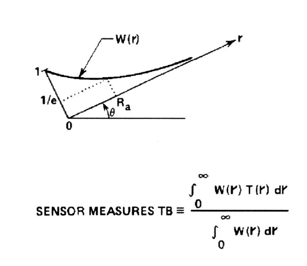
Figure 5. Brightness temperature measurement theory, for view along direction r inclined angle θ above horizon, showing weighting function W(r). At r = applicable range, Ra, W(r) = 0.37.
If
the entire emitting region were to change temperature,
TB would undergo a corresponding change. This is because each volume element would be emitting a fixed
ratio of
photons in relation to that for the original temperature.
But what happens if only some volume elements
change temperature?
The
weighting function W(r) can be used to calculate the
change in TB for a temperature change at any range increment. It is intuitively reasonable that the
equation in Fig. 5 can be used to calculate TB. Note that the "source function" is T(r), and it is weighted by
W(r) to yield an effective radiating temperature TB.
|
When
an exponential weighting function is applied to a linearly varying
source function, the weighted result equals the value of the source
function at the location where the weighting function = 1/e.
|
In
other words, if temperature varies linearly with range
(ie, if T(r) is a linear function
along the viewing direction), and if the Kv
of the medium is constant along the viewing direction,
then TB = T(Ra)!
Now
consider the case in which the temperature field is
horizontally stratified. It becomes
possible to transform from the range coordinate to a height coordinate,
according to: h = r * sin(θ). This leads to the concept of an
"applicable height" which varies with θ:
Ha = Ra * sin(θ)
The
source function is a linearly varying function of
height, and the weighting function will vary exponentially with height
if Kv
is constant with height, so it is possible to state
that:
|
When
air temperature varies linearly with altitude along the viewing
direction, and when absorption coefficient is constant along the
viewing direction, then T(h) can be derived from TB(θ)
by using the equivalence: h
= Ra * sin(θ).
|
When
the stated conditions exist, it is possible to
derive a profile of air temperature with altitude by measuring TB(θ),
provided a value for Ra can be
determined. The procedure is to first
derive TB(θ),
then
replot TB versus Ra * sin(θ)
and rename the plot as T(h).
Ra
is simply 1/Kv. Since Kv
in the 60 GHz region is a function of frequency,
pressure and temperature in the atmosphere (to first order), Ra can be
calculated from easily measured atmospheric parameters.
For example, referring to Fig. 2, while
flying at 10 km and operating a 60 GHz radiometer, Kv
»
2.0
[Nepers/km]. Thus, Ra »
0.5 km. If the
antenna is pointed through a range of elevation angles from -90 to +90
degrees,
it should be possible to estimate air temperature over an altitude
range of 1.0
km (from 9.5 km to 10.5 km).
The
remote sensing capability just described assumes that
T(z) is linear over an altitude region of unspecified extent; and it
assumes
that Kv
changes by only a small amount across the same altitude region. We will return to these assumptions, as well
as others not yet stated. For now,
however, it will be instructive to pursue the power of such a simple
radiometer
operated in an elevation scanning mode, with its TB output subjected to
such a
simple analysis algorithm.
In
describing something complex it is sometimes useful to
employ a series of explanations that begin with a very over-simplified
picture,
which can be replaced with more and more accurate representations later. Thus, I invite the reader to begin by
thinking of a microwave radiometer operating in the 60 GHz region, and
mounted
on an aircraft, as similar to a long stick with a thermometer on the
end that
is waved up and down in front of the aircraft.
Figure 6 conveys this idea.
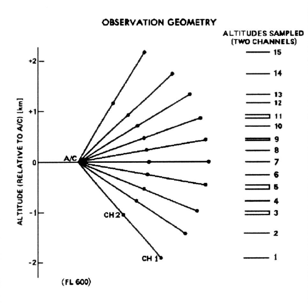
Figure 6. Microwave Temperature Profiler's viewing geometry, showing where air temperature measurements are "made" during each scan of 10 elevation angles.
This
figure is for the JPL Microwave Temperature
Profiler, MTP, which is mounted in NASA's ER-2 aircraft, also referred
to as
MTP/ER2. MTP/ER2 operates at two
frequencies, 57.3 and 58.8 GHz, called "channel 1" and "channel
2." When flying at 60,000 feet
altitude the applicable ranges for these channels are Ra = 2.5 and 1.5
km. In the Fig. 6 the "stick with a
thermometer
at the end" has these lengths, and it sweeps through a set of 10
elevation
angles during each scan. The
"dots" in the figure denote the "applicable locations" for
each of the elevations, for each channel. (On the right is shown how the redundant observables are
combined into a
set of 15 "independent" observables.)
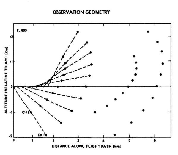
Figure 7. Location
of MTP air temperature sample locations after allowance for A/C motion.
The
next increment of realism to add to this picture is
to explicitly acknowledge that Kv
is not constant along the entire length of the viewing
direction. It only needs to be constant
for a distance of a couple Ra lengths in order to assume that the
weighting
function is approximately exponential. Slight departures from the exponential shape for the weighting
function
can be handled by calculating the exact shape of the weighting function
directly, according to (note use of "z" instead of "h" to
denote height):
W(z)
= e-τ
μ
* Kv(z)
* dz
(3)
where τ
= μ Integral [
Kv(z)
*
dz ]
and where μ =
1/sin(θ)
and
then using this weighting function to calculate
applicable height:
Ha
= Integral [
z * W(z) * dz ] / Integral [
W(z) * dz]
(4)
This
will provide an improvement over the assumption that
Kv
= constant throughout (which
would produce an exponential weighting function, which in turn would
have
permitted the use of the simpler expression Ha = sin(θ)/Kv).
The
next incremental improvement is to correct for any
"transparency" that may exist. A transparency correction is
needed for only those situations where the weighting function is
"long" and the viewing direction is at least a few tens of degrees
above the horizon. This may occur while
flying at a high altitude and observing at frequencies well off the 60
GHz
absorption peak. If the atmosphere is
not completely opaque along the viewing direction then TB will consist
of two
parts: an atmosphere part and a cold
space "cosmic background" part. For example, suppose the atmosphere was 1% transmissive, and
suppose the
atmosphere were at a uniform temperature of 260 K. Then TB would be 0.99 * 260 [K] + 0.01 * 2.7
[K], or TB = 257.4 [K]. (Note here that
I've adopted 2.7 K for the cosmic background brightness temperature;
there are
subtle second order effects requiring that a slightly different value
be used,
which are not worth getting into here). When the atmosphere is not opaque TB can be slightly less than
the
physical temperature of the atmosphere, and a small transmissivity is
then
required.
For
MTP it is necessary to apply transparency corrections
while flying above 60,000 feet, and then only to the TB measurements
where the
viewing directions exceed about 20 degrees above the horizon. Detailed calculations must be made for each
of the observables, ie, for each
channel, at each elevation angle, each altitude, and each air
temperature (and
lapse rate). This can take several weeks
of a person's time, so there's an incentive to minimize the amount of
transparency that must be applied (this entails carefully selecting
local
oscillator center frequency and IF passband shape to minimize the
amount of RF
response in the "wings" of the oxygen absorption spectrum.) It will probably always be the case that
transparency corrections will only be needed during flight at high
altitudes.
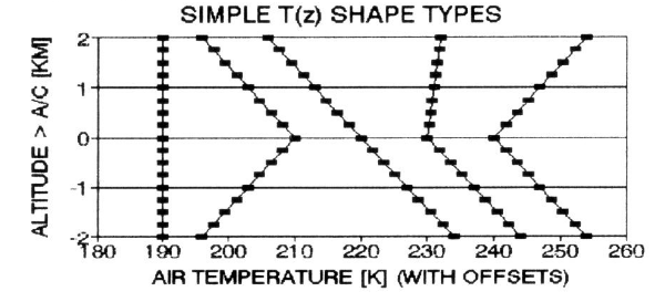
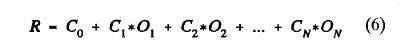
Figure 8. Altitude temperature profile shape types for which the "simple" procedure for converting TB(θ) to T(z) is fully adequate. The shape types are isothermal, IL top, featureless, tropopause, and IL base.
What
about the assumption requiring that the source
function, T(r), be linear with r? This
requirement could be met by a variety of altitude temperature profiles,
depicted in Fig. 8. But the five shape
types depicted are special cases since the aircraft will not often be
flying at
the altitudes of temperature inflections, with deep layers having
constant
slopes for large altitude regions above and below flight level. Figure 9 illustrates two cases of inversion
layer bases approximately 0.5 km above and below flight level.
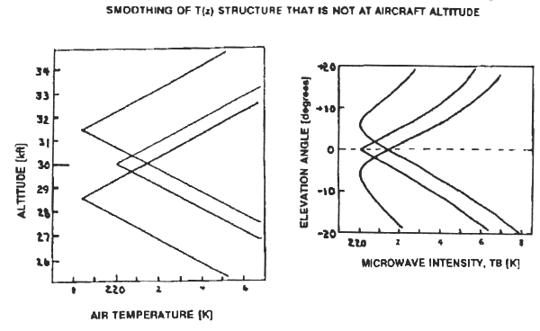
Figure 9. Examples of T(x) shapes with inflections displaced above and below aircraft altitude 0.5 km, for which the simple procedure for converting TB(θ) to T(z) is inadequate. Note the "smoothing" of observed TB(θ).
The
"rounded" TB(θ)
patterns in Fig. 9 show that the observed
profile will underestimate the extremes of air temperature at the
inflection
altitude. All sharp inflections not
close to flight level will be "rounded" and the altitudes of the
inflections will be displaced toward the aircraft (by small amounts,
not shown
in this figure). This illustrates the
major shortcoming of the simple procedure for converting observed TB(θ)
to T(z). It should be noted, however, that measured lapse rate at flight
level is
least affected for these cases.
I
believe that the details of the temperature structure
near the inflection altitudes is less important than other aspects of
the
temperature profile, which are acceptably represented by the simple
analysis
procedure. Usually the most important
thing about such T(z) structures is the mere presence
of the structure, and its altitude location in relation to
the aircraft.
Fig.
10, for example, shows a sequence of actual altitude
temperature profiles based on MTP/ER2 data which has been reduced using
the
simple data analysis procedure. Altitude
is resolved into rows 1100 feet apart (with the blank row representing
the
aircraft's altitude of 19.69 km), the horizontal temperature scale is
resolved
into 0.25 K columns, and each of the altitude temperature profile
sequences is
displaced 20 columns (5 K) to the right of its neighbor for clarity. The data were made while flying within an
inversion layer. The lapse rate at
flight level can be seen to vary, and the temperature contrast across
the
inversion layer also varies. For CAT
warning objectives it can be argued that the most important pieces of
information to be extracted from such a data set is that 1) the
aircraft is
flying in the middle of an inversion layer, 2) the lapse rate within
the
inversion layer is approximately +1.5 [K/km], 3) that the inversion
layer is
approximately 1.5 km thick, and 4) each of these properties is variable
on a
timescale of 14 seconds. This is a
significant amount of information, and it is all reliably obtainable
using the
simple procedure for converting TB(θ)
to T(z).
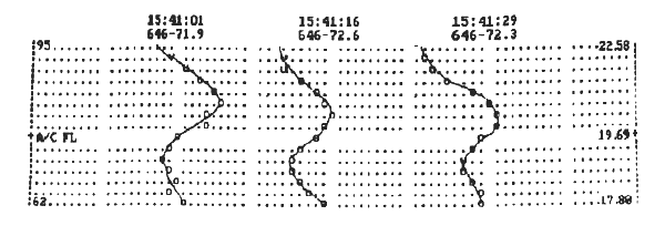
Figure 10. MTP
measured "altitude temperature profiles" obtained using the simple
procedure for converting TB(θ) to T(z). Each column represents 0.25 K, each row 1100
feet. Profiles are offset 20 columns. Note the changes in inversion layer properties.
Because
the analysis procedures used for this data were
"simple" it is not possible to believe the "softness" of
the temperature inflections at the base and top of this inversion layer. Also, it is likely that the inversion base
and top altitudes are slightly farther from the aircraft's flight level
than
implied by the observed profile. When
such details are needed, the more rigorous approaches (described later)
will
have to be employed. So far, these more
rigorous procedures (there are several) have just not been worth their
trouble
since they are significantly more laborious to set-up and use.
At
this point in the description of how microwave
observables are converted to altitude temperature profiles it is
possible that
"purist" readers will feel frustrated. The
transformation from "observable
space" to "reality parameter space" using the procedures
described so far appear to lack rigor! This is true, and in a later section I will describe several
more
rigorous treatments. However, I want to
state quite clearly that the simple
procedure for converting observables to altitude temperature profiles
works
quite well! All of my published MTP
results, for the ER-2 and all precursor instruments on other aircraft,
are
based on the procedures already described.
Air
Temperature Horizontal Gradients
The
previous sub-section describes how a 1-frequency
radiometer can be scanned in elevation angle to produce observables
that can be
combined to yield an estimate of "altitude temperature
profiles." It was also shown how
additional frequencies can be used to extend the altitude range of
these
profiles. This sub-section describes how
a horizontally-pointed radiometer can be used to estimate temperature
along the
viewing direction. For this application
it is necessary that more than one frequency be used.
When a sufficient sampling of frequencies are
used it is theoretically possible to determine air temperature at
several
locations along the viewing direction, and by differencing them it is
possible
to infer the existence of horizontal temperature gradients.
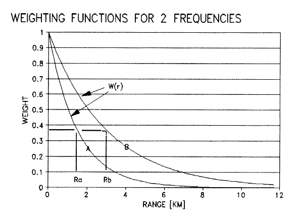
Figure 11. Weighting
functions for 2 frequencies having applicable ranges of 1.5 and 3 km.
Figure
11 illustrates the situation when two frequencies
are employed by a horizontally viewing radiometer.
Since air pressure is constant with range it
can be assumed that Kv(r)
is
constant versus r, which means that the weighting functions have
exponential
shapes. Channel A and B, in this
illustration, have applicable ranges that differ by a factor of two.
The
measured brightness temperatures for channels A and
B, TA and TB, will be the weighted average air
temperature corresponding to the weighting functions A and B. If air temperature changes linearly with
range then TA and TB will equal the air
temperatures at
the ranges Ra and Rb. This affords a
means for sensing the presence of a horizontal gradient of air
temperature
along the viewing direction. In the
above example, if air temperature varies linearly with range and is 5 K
colder
at r = Rb than at r = Ra, then the measured TB will be 5 K
colder
than TA. An abrupt change of
air temperature at a range of 3 km, for example, will produce a
measured
brightness temperature difference of about 3 K.
The
measured brightness temperature contrast is less than
the true air temperature contrast. The
next sub-section describes ways of recovering some of this lost
contrast.
Retrieval
Concepts: Backus-Gilbert
The
difference between the weighting functions in Fig. 11
is called an "averaging kernel."
Figure 12 shows the averaging kernel Aba(r).
What is the "meaning" of this
averaging kernel, and what is it good for?
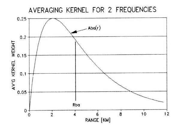
Figure 12. Averaging
kernel derived from weighting functions in previous figure. Applicable range is 4.1 km.
If
the areas
under the weighting functions A and B are designated by α
and β
(after normalizing to produce unity at r = 0), then
there is something special about the "artificially produced
observable," TBA,
defined by the following equation:
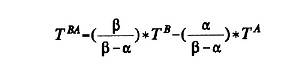
When
the two Kv
values are in the ratio 2 to 1, for example, then the
areas under the weighting functions are in the ratio 1 to 2, and TBA
= 2*TB - TA. The
"artificially produced observable" TBA is a linear
combination of the directly observed "observables" TA and
TB. Note that the sum of the
coefficients which "multiply" the directly observed observables add
up to 1! (This is an obvious
requirement, whose justification is left to the reader.)
With
TBA defined this way it is intuitively
clear that TBA is the brightness temperature that would be
observed
if a radiometer could somehow have the weighting function specified by
the
averaging kernel Aba(r). If a weighting
function like Aba(r) could magically be created, then TBA
would be
the "directly observed observable." As it is, we must perform the magic manipulation ourselves by
using TB
and TA along with the proper coefficients to infer the TBA
that would be measured.
This
manipulation to produce the equivalent of an
"averaging kernel weighting function observable" is widely used under
the name Backus-Gilbert retrieval to
infer information about a source function's value at a narrowly defined
range
region. I will use the term
"averaging kernel observable" to refer to this class of inferred
"observed" quantity. The
"applicable range" for the averaging kernel observable in Fig. 11 is
simply the averaging kernel weighted range, Rba. Note
that the function Aba(r)
"peaks" shortward of Rba.
The
multiplying coefficients used to convert the two
observables TA and TB to the averaging kernel
observable
TBA are -1 and +2 in the above example. Their sum is +1. Other combinations
that meet the "sum =
1" requirement can be used, but they will produce differently shaped
averaging
kernels. These differently shaped
averaging kernels are not "wrong," they may simply not be
"optimum."
"Optimum"
requires definition. Averaging kernels
that are "bunched
up" near their applicable range (Rba in the example) are more optimum
than
those which are "spread out." This subjective terminology can be made objective, but to do so
would go
beyond the scope of what is needed here.
It
can be said that the 2-channel radiometer in the above
example produces information about air temperature at three distances: Ra, Rb, and Rba (in increasing
distance). Other slightly different
definitions of the averaging kernel do not contain sufficiently
different
information to constitute being considered new air temperature
estimates.
The
shape of the averaging kernel in Fig. 12 may be more
"bunched up" near its applicable range compared with the weighting
functions in Fig. 11, but there still is something unsatisfactory about
the
shape. It would be good if the averaging
kernel shape were more impressively confined to a region near the
applicable
range. This is achievable, but more than
2 directly measured observables are required.
There
is a rule of thumb stating that "in the
limit" the half-response points of an ideal averaging kernel are at
distances of approximately 80% and 130% of the applicable range
(provided the
averaging kernel's applicable range is not near the ends of the set of
weighting function applicable ranges). A
sketch of an ideal, "in-the-limit" averaging kernel is shown in Fig.
13 using a thin line.
A
more realistic
averaging kernel shape is also shown in Fig. 13, by the thick line. In this case the 8 observable applicable
ranges are 1, 1.5, 2, 3, 5, 7, 10 and 15 km (note the approximate 1.5
ratio of
the sequence). The multiplying
coefficients used are +0.3, +7.9, -22.9, +21.5, -8.1, +4.6, -4.2 and
+1.9. This alternating sign pattern is
common, with
large absolute values for the observables whose applicable ranges are
close to
the resultant averaging kernel's applicable range.
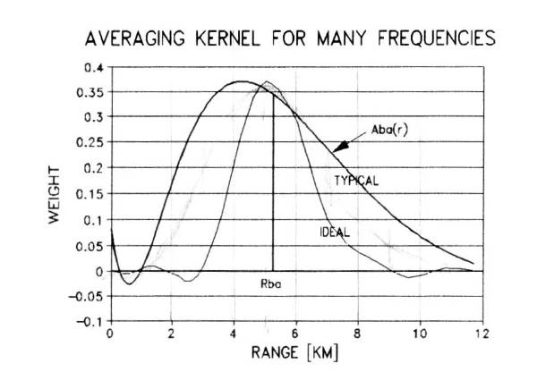
Figure 13. Improved
averaging kernel using 8 frequencies (thick line) and "many"
frequencies (thin line). Applicable range
is 5.3 km in both cases.
For
this specific set of 8 measured brightness
temperatures it is possible to construct an averaging kernel having an
applicable range of any value within the limits of the weighting
function
applicable ranges. The shapes degrade (i.e., begin to resemble the weighting
functions) for applicable ranges at the near and far limits of this
range
region, and the best looking shapes are always in the middle. The samples in Fig. 13 are for the middle of
the range of possible solutions.
Penalties
are paid for achieving range discrimination
using the averaging kernel concept. Observation noise is "amplified" since the averaging kernel
observable is the result of taking the difference between two large
numbers
(the sum of the terms with positive coefficients minus the sum of terms
with
negative coefficients). In the case just
described, with 8 terms, the averaging kernel observable can be
expected to exhibit
a stochastic uncertainty that is 34 times greater than for any of its
constituent measured observables. If
each measured observable has a noise uncertainty of 0.1 K, the
averaging kernel
noise uncertainty will be 3.4 K (for the 8-term case illustrated).
Even
more important than the amplification of stochastic
noise is the amplification of calibration uncertainties. It is typical for the final absolute
calibration of a radiometer to be uncertain by the amount 0.5 K. If each channel of an 8-channel radiometer
were uncertain by this amount the 8-term averaging kernel solution
would have
an uncertainty of a whopping 17 K! It is
forbidding to imagine how uncertain the "ideal" solution, with good
range resolution, would be. Clearly,
there are trade-offs. And each
radiometer system will require a tailored trade-off calculation that
incorporates knowledge about expected absolute calibration error,
stochastic
errors, and the need for good range resolution.
There
is a formalized procedure for handling the
trade-offs of observable uncertainty and range resolution that produces
coefficient sets that are optimum for any desired averaging kernel
applicable
range. I won't describe it here, because
there's an even better procedure for obtaining optimum coefficients: the "statistical retrieval
procedure" (to be described in the section after the next one).
Angle-Scanning
Inter-Channel Calibration
Before
describing the "statistical retrieval
procedure" this would be a good place to digress to explain why angle scanning is better than frequency
sampling. (The executive reader may
want to skip this
sub-section.)
The
explanations in the previous sub-section (including
Fig's 11 to 13) are for the "traditional" frequency
sampling observing strategy. That is, each observed
quantity comes from a separate radiometer channel. Most applications requiring the derivation of
air temperature versus range have really been attempts to derive air
temperature
versus altitude from a ground
station. Many observationalists have
built radiometers with many channels which have been mounted in a
zenith-fixed
position. Such systems suffer the full
impact of "calibration uncertainty amplification" when averaging
kernel techniques are employed. (The
same is also true when the "statistical retrieval procedure," to be
described later, is employed.)
Surfaces
of equal temperature are amazingly flat. This
fact can be taken advantage of by using
a single channel radiometer to do the job of several frequencies by simply angle scanning, as is done for each
channel of the MTP/ER2 instrument.
For
example, I will describe a ground-based radiometer
system called MARS, for Microwave Atmospheric Remote Sensor. MARS uses a 57.5 GHz radiometer to scan from
zenith to 5 degrees above the horizon, making measurements at 7
elevations. Each of the 7 measurements
produces a weighting function versus altitude
(note the transformation from range to altitude) with an applicable altitude given by "applicable range
times sine elevation." The
applicable altitudes for MARS span the range 120 to 1400 feet. The observed quantities are indistinguishable
from using a 7-channel radiometer pointed at zenith. But the angle scanning set of observables share the
same absolute calibration
uncertainty. Thus, they have a
greater amount of "shape information," the shape of the curve of
observed brightness temperature versus applicable altitude. Consequently, the single-channel, angle
scanning radiometer does a better job of sensing the presence of
altitude
temperature structure, and it is much less costly than a 7-channel
counterpart.
Since
the top altitude of 1400 feet is not high enough
for most uses, two additional channels are included in MARS. They also angle scan, from zenith to 25
degrees elevation. Provided the
frequencies and scanning angles are carefully chosen, as they were for
MARS,
such a hybrid angle scanning/frequency
sampling radiometer system can be "self inter-calibrating." Specifically, the 57.5 GHz channel's zenith
weighting function is identical to the 55.3 GHz channel's 25 degree
elevation
weighting function; and the 55.3 GHz channel's zenith weighting
function is
identical to the 53.9 GHz channel's 25 degree elevation weighting
function. By this means each scan of the
3-channel assembly provides sufficient inter-calibration to allow data
analysis
to force all observables to share the same calibration. This procedure assures that the shape of the
observables versus
applicable altitude is correct, or unaffected by calibration
uncertainties.
This
hybrid radiometer system also provides a less costly
way of providing a large dynamic range of applicable altitudes. The 3-channel MARS system measures brightness
temperatures with 15 weighting functions having applicable altitudes
that span
the range 120 to 6900 feet. That's a
dynamic range of almost 60 to 1! There
is no way a zenith-fixed, multi-channel radiometer system can produce
the same
dynamic range, or the same quality of inter-channel calibration.
For
the past 10 years I have promoted this observing
strategy. It has been demonstrated on
numerous
occasions using the MARS ground-based instrument, which is described
further in
a later section. We built an improved,
much more compact version, for the Army. The same concepts can be used in airborne radiometers that
endeavor to
derive altitude temperature profiles. Indeed, the MTP/ER2 instrument has two channels with several
overlapping
weighting functions (cf. Fig. 6).
For
angle-scanning multi-channel radiometer systems (used
to provide inter-channel calibration) there is no absolute calibration
amplification when deriving averaging kernel estimates of air
temperature. There is
stochastic noise amplification, but this can be made quite small by
using wide
bandwidths, low-noise amplifiers, or by averaging measurements. The practical limits to using averaging
kernels approaching the "ideal" shape are set by other factors. They are set, for example, by the accuracy
with which weighting function shapes can be assumed
- due
to slight errors in observing frequency, or uncertain knowledge of the
physical
constants producing absorption coefficients, Kv,
or slight inhomogeneities in the Kv(r)
profile (caused by aerosols, water vapor, clouds,
etc).
The
angle-scanning multi-channel radiometer system
concept cannot be used for improving horizontal gradient measurements. Such systems will probably always be subject
to the full impact of absolute calibration amplification.
Statistical
Retrieval Procedure
The
"statistical retrieval" (SR) procedure is a
favorite method for converting remotely-sensed observables to desired
physical
properties, called "retrievables." It is an all-purpose tool that has found applications in many
fields
besides remote sensing. The same factors
that render it powerful also render it dangerous on occasion. It must be used carefully, with awareness of
limitations and pitfalls. Since each
situation can usually be served by many possible retrieval procedures,
it is
important that careful thought be given to their strengths and
weaknesses in
relation to the intended use. Sometimes
the SR procedure may not offer the best match to the user's needs. This sub-section will briefly sketch how the
procedure works, and highlight its main strengths and weaknesses. (The executive reader can read this
sub-section "quickly.")
It
will be useful to think in terms of "reality
space" and "observable space." In reality space are the things we want to have values for, such
as air
temperature at a specific altitude (or specific range). In observable space are the things our
instruments measure, such as brightness temperature at specified
frequencies
and viewing directions. Both
"spaces" can have any number of dimensions. It
is straightforward to calculate where in
observable space a set of measurements should be if we first specify
the
reality space location. This assumes, of
course, that we have complete knowledge of the physics governing thermal
emission
and intervening absorption and scattering. There are no ambiguities transforming in this direction. For every hypothesized location in reality
space our physical model "maps us over" to only one location in
observable space, as illustrated by situations A, B and C in Fig. 14
(note that
realities B and C map to the same location in observable space).
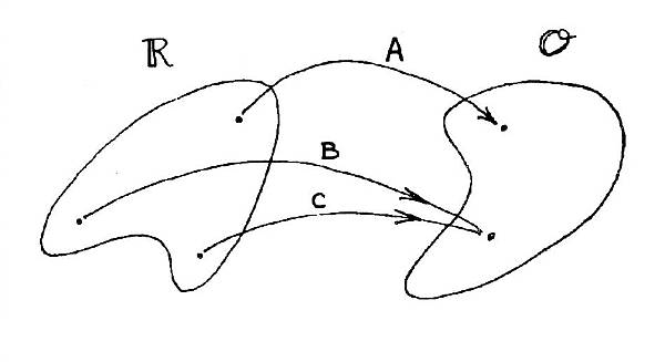
Figure 14. Mapping
over from Reality Space to Observable Space.
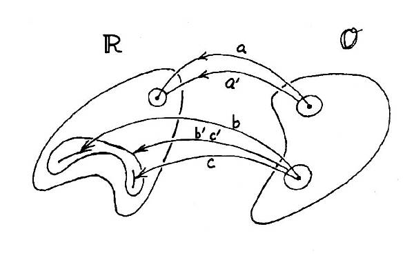
Figure 15. Mapping back from Observable Space to Reality Space.
It
is not
straightforward "mapping back," going from observable space to
reality space. Indeed, there are
ambiguities,
in which one location in observable space maps over to many points in
reality
space, as illustrated by situations "b" and "c" in Fig.
15. This situation can occur when
observables are integrated quantities, like brightness temperature. When observing uncertainties are taken into
account we are dealing with mapping back from areas in
observable space to areas
in reality space, as shown by a' in Fig. 15. For the situation in which more than one reality produces
identical (or
nearly identical) observables a small area in observable space can map
back to
a large area in reality space. This is
depicted in Fig. 15 as situation b'c'.
These
examples illustrate how care must be taken in
transforming observables to an
inferred reality. It is
necessary to assure that the
"best" solution is obtained, and to assure that formal uncertainties
take proper account of the mapping ambiguities. Sometimes the "best" solution is one that is known to occur often in reality, even though its
corresponding observables are no better than those corresponding to
some
alternative reality. The SR procedure
can be used to do a powerfully good job of this.
The
SR procedure consists of two parts. First
an archive is created, consisting of
paired sets of realities and observables. For example, we might begin with 100 radiosondes. For each radiosonde we note the values of the
parameters we want to retrieve and we calculate what the observable
values
should be (using a good physical model and a perfect measuring
instrument). This will produce 100 sets of
observable
locations paired with their corresponding reality locations. (The use of the term "location" is
merely a shorthand way of referring to a set of values, corresponding
to a
"vector" in either observable or reality "space.") In the example just cited, the observables
are "simulated" using a believable physical model.
It
is also possible to use real measurements in the SR
analysis, perhaps taken specifically for creating an SR archive. Using real
observables in the SR analysis is a variant which is less commonly used
due to
the greater cost compared with using computer simulations. It is a superior option that may justify the
additional cost since real observables contain idiosyncracies of the
measurement system. However, the
retrieval coefficients obtained using real observables might not be
useable
with an upgraded observing system with fewer, or different,
idiosyncracies.
The
second part of the SR process is to calculate
"retrieval coefficients" that will enable a transformation to be made
from observable space to reality space. The transformation is made using a simple linear
series:
where
R is one
of the retrievables, Oj are
the observables, and Cj
are the retrieval coefficients (and there are N
observables). Any set of
values for Cj will
transform from observable space to reality space, but there is one set of values for the coefficients
that will do this job with a minimum RMS residual between the archive
reality
values and the retrieved reality values. The trick is to find that one optimum set of values for Cj so that this minimum
variance is achieved.
The
set of C
values is a vector (of dimension N+1). It is theoretically possible to locate the
desired location in "N+1"-dimensional
space by a "brute force" method of searching all reasonable
combinations for Cj-values
and keeping track of the RMS variance performance for each. But there's a better way to locate the best
set of values for the C vector. It
requires that two covariance matrices be
calculated.
First,
the matching sets of observable and reality
vectors must be "conditioned," or expressed as differences from their
ensemble averages.
Then
the "cross-covariance" and
"auto-covariance" matrices are calculated, SRO
and SOO. SRO
contains information on all the correlation combinations between the
conditioned retrievables and observables (summed over all simulation
cases),
and SOO consists of all
the correlation combinations between the various observables (summed
over all
simulation cases). The SOO
matrix is then inverted, and multiplied with the SRO matrix, producing a
matrix that is the desired C matrix
of optimum retrieval coefficients. If
there are i retrievables (reality parameters) and j observables, then
the C matrix is a "j by i"
matrix. It is possible to make
allowances for a priori measurement
uncertainties by creating an "error matrix" and adding it to the SOO matrix before it is
inverted.
The
reader who wants details about any of these matrix
manipulations is referred to other more lengthy treatments, such as
that of
Westwater (1972). The already lengthy
description given here is meant to convey a flavor for what "goes
into" the derivation of SR coefficients. The astute reader will recognize that virtually any measurable
quantity
can be used as an observable. For
example, the "price of eggs" might have a useful correlation with air
temperature at a specific altitude, and the formalism can accommodate
the
inclusion of this and other more outrageous observables!
It
is important to be mindful of some strengths and
weaknesses of the SR procedure. The SR
coefficients provide a minimum variance between the archive
retrievables and
the retrieved retrievables. If the
archive contains many representations of a particular situation, that
situation
will be "favored" in subsequent uses of the SR coefficients. Equally good solutions will be
"unfavored." This may be
considered a strength, or a weakness, depending on the nature of the
observing
situations for which the statistical retrieval coefficients are to be
used, and
depending on the objectives. It is a
strength when future observing situations are similar to the archive
giving
rise to the SR coefficients and when the proper retrieval of common
situations
is to be emphasized. It is a weakness
when future observing situations will not
be similar to the archive, or when the proper retrieval of uncommon
situations is to be emphasized.
The
SR procedure is only valid for the range of reality
situations encompassed by the archive used to generate the coefficients. When novel conditions are encountered, or a
new environment is entered, there is no guarantee that the retrieved
reality
will be reasonable. If this can be
anticipated it is sometimes possible to attempt to allow for this by
artificially supplementing the archive with situations that endeavor to
include
the unusual or novel conditions. The
"wider" the archive the poorer the performance in the most common
reality area. So there are trade-offs in
trying to allow for too many unusual situations.
Bracewell
Retrieval Procedure
The
radio astronomer Ronald Bracewell employed an
iterative procedure for reconstructing brightness temperature
distributions on
the sky from beam-smoothed measurements of intensity versus sky
location. I later adapted these procedures
for
sharpening 2-dimensional maps of the moon's microwave brightness
temperature
distribution. The method is extremely
simple, and I will describe the procedure for recovering 1-dimensional
structure of any source function from observations that are smoothed
versions
of the source function.
Bracewell's
method for extracting structure involves the
observed distribution of anything versus something else. There is a true source function (the thing we
want) and a measured function (the thing we observe).
During the Bracewell iterations we
hypothesize a source function and calculate an observed function using
an
adopted smoothing function. For the case
of extracting spatial structure the smoothing function would be the
antenna
pattern and the source function is the true distribution of intensity
versus
angular location. For the case of
extracting air temperature versus range the smoothing function would be
the
observable weighting function and the source function would be the
profile of
air temperature versus altitude.
Figure 16. Distribution
shapes during the first iteration cycle of a Bracewell procedure for
recovering structure.
The
first step is to adopt the observed function as a
hypothetical true function. This
hypothetical true function is smoothed using the known smoothing
function, and
the resultant smoothed function is compared with the measured function. If agreement is "adequate," the
procedure stops and the hypothesized true function is accepted as true
(even
though no adjustments had been made). No
adjustments are needed when there are no "sharp" structures in the
true function (causing the observed function to equal the true
function).
If
the hypothesized function produces a predicted
hypothesized observed function
that departs significantly from the actually
observed function, then an
adjustment to the hypothesized function is required. A departure
function is defined as the "predicted hypothesized observed"
function minus the "hypothesized" function. This
departure
function is subtracted from the hypothesized function to produce a
new
hypothesized source function. This completes
one iteration cycle. The iterations are
performed until the departure function
is "acceptable." It is
important to "know when to stop" with the iterations. Stopping too soon produces a solution that is
too smooth, with unextracted structure "in" the observables. Stopping too late leaves unreal structure in
the solution, created by the magnification of observable noise.
In
computer simulations of spatial structure recovery,
with hypothetical true functions and typical observable smoothing
functions and
observable noise, I have found that approximately 5 iterations is often
close
to optimum. When the true function does
not contain high spatial frequency components the solution stabilizes
(successive hypothesized functions do not change) after fewer
iterations. When the true function is
"rich" in
high spatial frequency structure, however, solutions do not stabilize
and noise
magnification can degrade solutions past 5 or 6 (depending on the
signal to
noise ratio, etc).
There
are Fourier decomposition ways of understanding
what the Bracewell method is accomplishing, which are probably obvious
to the
astute reader. In fact, the reader may
wonder why it is not better to decompose the observed function into its
Fourier
components and multiply them by the inverse of the amplitude of the
corresponding Fourier components of the known smoothing function to
obtain a
solution function. Indeed, this can be
done (after proper "windowing" of the observed function), and quite
extensive and sophisticated procedures for sharpening structure have
been
developed by many workers in many fields.
I will not describe them here because the Bracewell procedure is
computationally simpler, its implementation is straightforward, and it
serves
to illustrate the concept.
In
using the Bracewell method for recovering structure it
is necessary to assume something about the observed function beyond the
edges
of the observed field. In some cases the
observed levels have reached zero at the edges and it can be assumed
that the
observed function remains at this value for all unobserved locations. Other situations do not lend themselves to
such easy assumptions. For the situation
of measuring air temperature versus altitude it is necessary to assume
that the
unobserved observable function is a simple extrapolation of trends just
inside
the observed boundaries. When this
assumption cannot be made, or when the unobserved region cannot be
represented
properly, the Bracewell solution will not be valid near the edges.
The
Bracewell method is useful when the statistical
method cannot be used (because there is no archive of actual past
conditions
from which to create retrieval coefficients), or when it is "too much
effort" to calculate statistical retrieval coefficients. It's main value is speed and simplicity, and
a 1-iteration use of the Bracewell method can be used to estimate if
there is
"recoverable" structure in the observables that may warrant use of a
more powerful method.
Mutational
Retrieval Procedure
Biological
evolution is a process of
"proposing" solutions and having some outside force
"select" winners. The winners
of each generation are the starting point for "proposing" a suite of
slightly altered solutions for the next generation of selection. Mutation is the process of creating slight
alterations. As this process evolves
there is often an increasing "match" between the "resultant
observed properties" and something related to the selective forces. There are some striking resemblances between
biological evolution and a novel retrieval process called "mutational
retrieval." (The differences are
just as interesting, but well outside this tutorial's realm of
relevance.)
A
temperature profile (the concept also applies to
temperature versus range) can be described in terms of a small set of
parameters, such as temperature at one location, gradient at that
location,
location of a temperature distortion (such as an altitude temperature
profile
inversion layer), and properties of this distorted region, etc. The user of the mutational retrieval
procedure must give considerable thought to the selection of as few
descriptive
parameters as possible. It is desirable
to create as much "orthogonality" as possible (so that altering one
parameter
will not have effects similar to those of another parameter). I invite the reader to think of these
descriptive parameters as "genes."
An
observing instrument doesn't observe the parameters,
only the effects of the parameters;
or the aggregate effects of all the parameters working together. The sum of the effects of all the parameters
is a temperature profile. Only after
some thought is it possible for the physical scientist to view the
profile as
something produced by the sum of effects of individual parameters with
specified values. The parameters are a
very useful conceptualization even though they are never directly
observed.
Not
only does the physical scientist never directly
observe the parameters that determine a temperature profile, he never
observes
the temperature profile either. What is
observed is merely a set of "observables" which are related
to the temperature profile. The
observables are related to the
temperature profile by the properties of measuring instruments.
This
is analogous to stating that the forces of selection
do not interact directly with an individual's genes, nor with the
genotype (the
sum of all genes that influence anatomy, physiology, and behavioral
predispositions). Rather, the selection
forces interact with a "phenotype," the combined expression
of the genes influencing anatomy, physiology and
behavior. The relation has been
described as G + E = P, or Genotype plus Environment produces Phenotype. Phenotypes determine the fate of the
underlying genotype elements: the
genes.
The
goal of the mutational retrieval procedure is to
derive a set of values for parameters describing a temperature profile
versus
altitude (or temperature versus range, etc) which provide a good match
to
observed quantities. The process is
iterative, somewhat like the Bracewell method. An initial set of parameter values is chosen. Although it is not critical which
initialization is chosen, solutions are obtained faster by cleverly
converting
observed quantities to initial parameter values. The
chosen parameter values are used to
specify a complete temperature profile (or whichever source function is
appropriate). This temperature profile
is then used to calculate observed quantities.
The
next step is a comparing process. The
"predicted observed" quantities
are compared with the "actual observed" quantities, and the
discrepancies are used to calculate an RMS fit. A "figure of merit" is calculated which can contain a
priori information about expected RMS
fit, expected magnitude of lapse rates (it can penalize super-adiabatic
lapse
rates, for example), or anything else which brings in outside
"knowledge." The figure of
merit value is stored along with the parameter values which produced it. (This is analogous to the selective forces
"measuring" the merits of an individual and noting which constituent
genes make up the individual's genotype.)
Parameter
mutations are next generated (analogous to
genetic mutations). It is important to
perform mutations on the right number of parameters. Experience has shown that at least two
mutations per "generation" is better than just one (some locations in
parameter value space cannot be reached by following figure of merit
gradients
unless two or more parameters are allowed to vary). Experience has also shown that mutations
performed on all parameters is inefficient (payoffs can't be accurately
ascribed when too many parameters are varying at the same time). For altitude temperature profiling, where
approximately 8 parameters are involved, I have found that 2 mutations
are
close to optimum. Mutation amounts must
be pre-specified (other dynamics are possible). As a result of this mutation cycle, an "offspring" is
produced!
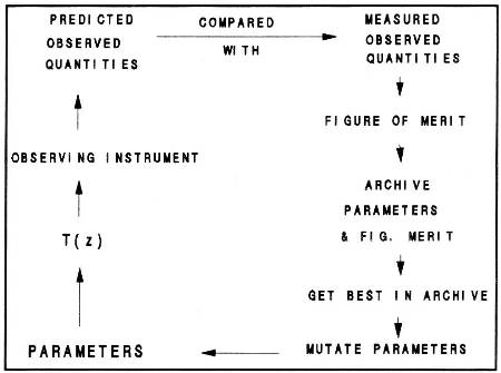
Figure
17. Flow of operations in performing "mutational
retrieval." Begin in lower-left corner; end when "Figure Merit" is
acceptable.
The
new ("offspring") parameter set is run
through the previously described cycle of "temperature profile
generation" and "figure of merit assessment." If
the offspring's figure of merit is better
than the "parent's," the offspring parameter set becomes the new
"parent" for the next iteration. If, on the other hand, the parent's figure of merit is better,
the
parent remains a parent for the next iteration.
After
each iteration, if the figure of merit exceeds a
threshold (set beforehand) the evolutionary search ends and the winner
is
declared! This process can produce quite
good agreement in "observable space." Since sharp structures composed of straight-line segments are
indeed a
property of real atmospheres, and since sharp structures composed of
straight-line segments are easily produced with parameters describing
temperature profiles, some remarkable structure recoveries are
achievable using
the mutational retrieval procedure.
Computational
speed is one potential limitation for this
method, however. This is intuitively
understandable considering that an 8-parameter temperature profile
representation requires that an 8-dimensional parameter space be
searched for
an "optimum" solution. In my
experience (with a 20 MHz PC clone with an 80387 microprocessor) it is
possible
to find a solution in 10 to 20 seconds (involving 50 to 100 "tries"). A 80486 computer should find solutions in
less than 5 seconds.
The
down-side of the mutational retrieval procedure is
that an efficient and accurate use of it requires that many subtleties
be
overcome. It is not a solution for
everyone as it must be implemented by someone experienced in the
"art."
PREVIOUS
APPLICATIONS DESCRIPTIVE REVIEW
Microwave
radiometric studies of the atmosphere can be assigned to the
following three application categories: 1) ground-based remote sensing of atmospheric properties, 2)
satellite-based remote sensing of atmospheric properties, and 3)
aircraft-based
remote sensing of atmospheric properties. The above sequence approximates the order in which these sub-discipline began,
and it
is ironic that aircraft applications followed
satellite usage. Ground-based systems
have been constructed since the late 1960s, satellite payloads for
earth
studies began in the mid-1970s, and the first aircraft instrument was
flown in 1978
(
Two
groups have dominated ground-based temperature profiling work: NOAA's Wave Propagation Laboratory (headed by
Ed Westwater), and NASA's JPL (headed by Bruce Gary). The early work in this field was done by the
NOAA/WPL group (from the late 1960's to the early 1970s). During the late 1970s the two groups
collaborated closely, since WPL was weak in hardware (where JPL was
strong) and
JPL was weak in retrieval theory (where WPL was strong).
Since the early 1980s, as the two groups
strengthened their respective weak areas, there has been a lessened
need for
collaboration.
I
will review radiometer systems built by the JPL group because I am
familiar with them and they adequately represent the flavor of
capability
improvements during this period. It
might be of interest to note that there are some minor "philosophical
differences of approach" between the two groups which can be accounted
for
by the slight differences in goals and previous capabilities within the
WPL and
JPL environments. The WPL group
emphasizes large, stable systems that are meant to take data in one
location
for years at a time, while the JPL group emphasizes small, portable
systems
that can be deployed easily at remote locations and supported by field
personnel. It is not surprising that
JPL's approach emphasizes smallness, considering JPL's history of
building
satellite instruments.
Since
airborne temperature profiling has been conducted by only the JPL
group, all examples in this category will be from work done by us
(since 1977).
Ground-Based
Temperature
Profiler MIST
JPL
built a ground-based temperature profiler in 1975 to study the
feasibility of placing microwave temperature profilers on deep ocean,
moored
data buoys for the purpose of supplementing the National Weather
Service's
radiosonde network to improve weather forecasts. Measurements
were made at Point Mugu, CA in
1976 in collaboration with NOAA/WPL, showing that air temperature and
vapor
profiles could be inferred using a 3-frequency, angle-scanning
radiometer. MIST operated at 22.3, 31.4,
54.0, 55.3, and
57.5 GHz.
In
1977 the MIST system was deployed aboard the weather ship Quadra,
which was stationed at a fixed location in the middle of the
Measurements
were made again in 1978 with the same instrument at the
Boulder Atmospheric Observatory 1000-foot atmospheric research tower,
during
the
Ground-Based
Temperature
Profiler MARS
JPL
built a Microwave Atmospheric Remote Sensor system, MARS, for
participation in EPA's 1980 PEPE (Persistent Elevated Pollution
Episodes)
experiment. After 5 days of data in
Croton, OH, MARS was struck by lightning, which terminated the MARS
participation in PEPE.
MARS
was repaired, and in March of 1983 it was deployed at
MARS
was operated at
Ground-Based
Temperature
Profiler BUOY
JPL
built a very compact unit combining a temperature profiler with a
water vapor and liquid (cloud) water radiometer intended for
installation on a
NOAA data buoy. It was to telemeter data
via geosynchronous satellite to a Weather Service forecast center. NOAA administration changes canceled plans to
follow through with the implementation of the radiometer on a buoy, and
it was
decided to test the system at
Ground-Based
Temperature
Profiler PMTP
JPL
constructed a compact microwave temperature profiler, called Passive
Microwave Temperature Profiler, or PMTP, which was delivered to the U.
S. Army
in 1988. It uses 4 frequencies from 51
to 58 GHz, and scans through 5 elevation angles from 9 degrees to
zenith. The 51 GHz channel serves to
monitor cloud
liquid content (a novel idea which no other temperature profiler
incorporates),
while the other three channels measure the temperature profile. This radiometer system is probably the best
portable
microwave temperature profiler in existence.
Ground-Based
Temperature
Profiler MTP/DOE
The
MTP instrument that is usually installed in the ER-2 aircraft was
modified temporarily for ground-based use for a 1991 March deployment
in
Airborne
Microwave System
MTP/CV990
The
first airborne microwave temperature profiler instrument, MTP/CV990,
was built by JPL in 1978 and installed in NASA's CV-990 "Galileo II"
(
MTP/CV990
is a modified version of the engineering model of the Scanning
Microwave Spectrometer (SCAMS), the flight model of which flew in the
NIMBUS-6
weather satellite. MTP/CV990 operated at
55.3 GHz, and scanned from 16 degrees below to 20 degrees above the
horizon
every 17 seconds. A microwave
"transparent" window had to be 1-inch thick to support cabin to
outside pressure differences, and even with anti-reflection grooves on
both
sides the window losses were 6% (3% due to absorption and 3% due to
reflections).
This
first flight series with an MTP instrument showed how useful MTP
could be in locating the altitude of the tropopause, where most
commercial
aircraft CAT is encountered. These
flights also provided evidence that inversion layers were also sites
for CAT
production. MTP/CV990 data was used to
produce a first-ever time-lapse movie of airborne ATP shape variations.
Airborne
Microwave System
MTP/C141
JPL's
next MTP instrument was built for NASA's C-141 Kuiper Airborne
Observatory (
Approximately
450 flight hours of measurements were obtained during the
years 1981 to 1985. Approximately 15% of
the flight data was near the tropopause, and it was determined that
there was a
greatly enhanced probability of encountering CAT during flight near the
tropopause (19% of 10-minute segments contained moderate or greater
CAT)
compared with flight in the troposphere (2.7% CAT) or stratosphere
(1.7%
CAT). Furthermore, two tropopause
"altitude temperature profile" shapes had different CAT
probabilities: the simple 2-segment
shape had a 13% probability of CAT whereas the 3-segment, inversion
layer shape
had a 24% probability of CAT.

JPL's
third MTP instrument is called MTP/ER2. It
was installed in NASA's ER-2 aircraft in
1985. The section "Altitude
Temperature Profiles" (pp 7-9) describe some aspects of MTP/ER2. It was used in the 1987
Stratospheric/Tropospheric Exchange Project, STEP, the 1987 Airborne
Antarctic
Ozone Experiment, AAOE, and the 1989 Airborne Arctic Stratospheric
Expedition,
AASE. At the present time this is the
only airborne atmospheric temperature profiler in use (since the two
predecessor MTP instruments have been "retired"). An
upgraded version of it will participate in
the 1991/92 "Airborne Arctic Stratospheric Expedition II," AASE II,
to be based in
The
entire instrument weighs 58 pounds, much of which consists of
1984-vintage power supplies (which are now being replaced with lighter
ones). MTP consists of two units: a sensor unit, weighing 10 pounds, and a data
unit, which is in the process of being lightened to an estimated 35
pounds
(including 15 pounds of power supplies). The dimensions are 13 x 7.5 x 5 inches for the sensor unit, and
18 x 14
x 9.5 inches for the data unit (the new data unit design is 17.5 x 8.75
x 7
inches).
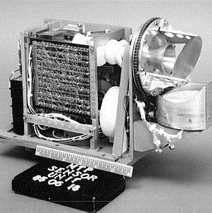
Figure
19. This MTP has flown in NASA's ER-2 aircraft
since 1985. It is more compact than the
earlier C-141 MTP, because it employs a smaller horn and a shaped
reflector which scans.
The
sensor unit consists of a scanning shaped reflector and horn
antenna, a microwave mixer operated in a total power mode, an IF
amplifier and
detector, and a voltage-to-frequency converter. Two local oscillators are turned on in turn, operating at 57.3
and 58.8
GHz. The IF bandpass has been 190 to 390
MHz during previous deployments, but it now is 265 to 375 MHz. A noise diode is injected between the horn
and an isolator, and provides a calibration signal of approximately 50
K. The double-sideband noise figure is
approximately 4 db, which produces a stochastic noise level of 0.12 K
for each
255 millisecond reading. Baseline
"wander" adds a component of approximately 0.2 K to the stochastic
noise, producing a net RMS uncertainty of 0.3 K. The
accuracy
of these readings is estimated to be 0.5 K.
The
horn antenna/shaped reflector assembly provide a beamwidth of 7.5
degrees (FWHM). The beam is scanned
through the following sequence of 10 elevation angles every 14 seconds: -50, -35, -22, -11, 0, +10, +20, +31, +44,
and +60. At each elevation angle
255-millisecond readings of the total power radiometer output are made
at both
frequencies. Each 14-second cycle
includes readings taken while viewing an ambient calibration target. An inclinometer is read prior to each scan to
provide an elevation angle offset which corrects for aircraft pitch
changes. A vertical accelerometer is
located in the data unit, and values from filtered maximum and minimum
excursion circuits are recorded. Aircraft synchro signals convey pitch, roll, and pressure
altitude
information to the microprocessor in the data unit. A microprocessor records the radiometer
readings, instrument temperatures, aircraft synchro signals, and clock
readings. The recording medium has been
a cassette tape unit, with a 0.5 Mbyte capacity (good for an 8-hour
flight). We are currently installing a
40 Mbyte hard disk removable recording unit.
Other engineering details can be found in Denning et
al (1989). The first
published description of MTP results can be found in
MTP
data have been presented in several forms, and each is useful for
different things. The most
straight-forward form is an "altitude temperature profile," or
ATP. Figure 10 is a sample of an
ATP. Successive ATP traces are offset by
specified amounts along the x-axis, and a glance of such a presentation
shows
whether interesting vertical temperature structures are present and if
they are
changing. Passage through the tropopause
is easily noted from an ATP presentation. The presence of inversion layers are also easily noted, and
estimates
can be made of the altitude of the inversion layer's top or bottom.
Another
form for presenting MTP data is a simple plot of lapse rate, LR,
versus time. Figure 20 plots LR versus
time for a flight that went from
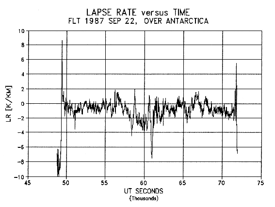
Figure
20. Sample MTP plot of lapse rate versus time
for a flight over
Another
form for presenting MTP data is something that can be called an
Isentrope Altitude Cross-section, or IAC.
To understand an IAC it is necessary to first understand the
atmospheric
properties "potential temperature" and "isentrope."
Potential temperature is a conserved property
of air parcels (meters to kilometers in size); it is the temperature an
air
parcel would have if it were "brought to" the 1000 millibar altitude
adiabatically (without allowing energy to enter or leave the parcel). The potential temperature of air can be
calculated by the formula:
θ
= T * (1000/P)0.27
An
isentrope is a surface of the atmosphere having the
same "potential temperature."
An IAC is obtained by calculating the altitudes of specific
isentrope
surfaces versus flight time, or the corresponding ground-track location. Since an aircraft's ground track is not
always a straight line actual cross-sections are often referred to as
"curtain cross-sections." An
IAC, therefore, can be more accurately described as an "isentrope
altitude
curtain cross-section."
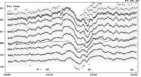
Figure
21. Sample IAC, Isentrope Altitude
Cross-section, obtained from the MTP/ER2 instrument, showing a
"mountain wave."
Figure
21 is a sample IAC. It was the first IAC
produced, during the
1987 AASE mission to
Since
potential temperature is "conservative,"
isentropes can be used to locate streamlines for air motion (provided
the IAC
is in a plane approximately parallel to wind vector). The isentropes in Fig. 21 imply parcel
cooling (during the upward displacements) of as much as 6 K, and
warming
(during the downward displacements) of the same amount. If the frost point depression is less than
the amount of the cooling, then a cirrus lenticular cloud will form at
the top
of the upward isentrope displacement. This phenomenon was documented during another flight over the
Data
acquired by the MTP/ER2 instrument was used to
derive a method for determining vertical wind shear, VWS.
VWS can be combined with lapse rate to infer
the value for the Richardson Number, which is a key atmospheric
property for
predicting CAT. The procedure for doing
this is the subject of a NASA patent application.
Airborne
Microwave System MTP/DC8
Currently
under construction, the JPL-built MTP/DC8 will
be installed in NASA's DC-8 research aircraft in October, 1991. Figure 22 is a sketch of the instrument. It will be a "many frequency"
radiometer, since it will be able to tune continuously between 55 GHz
and 59
GHz. In this band there are, in effect,
only 7 useable frequencies since it is only useful to set the local
oscillator
to frequencies in the valleys or peaks of the oxygen spectrum. MTP/DC8 will scan from nadir to zenith in
approximately 15 seconds.
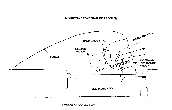
Figure
22. Sketch of MTP/DC8, looking down. MTP is installed in a window frame on the left side of the
DC-8 aircraft.
Simulations
show that this instrument will be able to
produce useful "altitude temperature profiles" extending from 4 km to
about 30 km. Figure 23 shows predicted
performance for altitudes above flight level (assumed to be 12 km).
The
MTP/DC8 data will be used during the AASE II mission
in 1991/92 to: 1) locate altitudes where
it is cold enough for PSCs to form, 2) assist in measuring potential
vorticity
(to locate the polar vortex boundary), and 3) study characteristics of
the
mesoscale up and down displacements that may influence PSC particle
size
distributions.
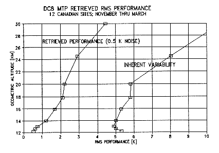
Figure
23. Predicted RMS uncertainty of retrieved air
temperature using the MTP/DC8 instrument.
The
newest MTP instrument is in design and is scheduled
for delivery to Rockwell International. Functionally, it will be very similar to the MTP/DC8 instrument;
but in
physical layout it will be more like the existing MTP/ER2. It will be capable of continuous frequency
sampling in the interval 55 to 59 GHz, using a VCO (voltage control
oscillator)
under computer control.
During en route flight it will scan a
7 degree
beam from nadir to zenith in 15 seconds. At each viewing direction it will sample a set of 5 to 7
frequencies,
and produce ATPs (altitude temperature profiles) that span 6 to 13 km
(for an
assumed flight level of 11 km). (It is
not necessary to determine the ATP above this region since step climb
possibilities are limited to 1 or 2 km above en route
flight level; and knowledge of profiles beyond several km
below flight level are not useful). The
intended use of MTP/RKW during en route
flight is to provide warnings of CAT, as well as altitude guidance away
from
the CAT.
In
the terminal area the MTP/RKW will scan a smaller
range of elevation angles but sample the full range of frequencies in
an
observing sequence designed to optimize the measurement of 1) lapse
rate near
flight level, and 2) horizontal air temperature gradients ahead of the
aircraft. The intended use of this data
is to assist in providing warnings for "low altitude wind shear,"
LAWS.
Airborne
Microwave System MTP/MMIC
It
is anticipated that future versions of the MTP will
incorporate MMIC (microwave monolithic integrated circuit) technology. This will be especially important for the
design of light weight and low cost MTPs for use in commercial aircraft
(where
cost and reliability are important) and unmanned aerial vehicles, UAVs
(which
have modest payloads). Without using
MMIC techniques an MTP could be built that would weigh approximately 10
pounds. We anticipate that by using
MMICs it will be possible to build an MTP weighing 1 or 2 pounds (plus
the
fairing and computer). Such a system
would employ a MMIC radiometer and a MMIC electrically-steered antenna. The cost for MTP/MMIC systems would be much
less than non-MMIC MTPs, perhaps $5000 instead of $200,000.