Links internal to this web pageAt my southern observing site the star that Pluto occulted exhibited a 23 ± 4 % fade during the March 18, 2007 occultation. This star flux loss amount is based on measurements of Pluto and the occulted star made one Pluto rotation after the occultation, showing that the star's brightness was ~33% of the total flux (Pluto plus star). The measured occultation duration was 5.3 ± 0.7 minutes . If the center of Pluto's disk had occulted the star the mid-occultation star flux would have dropped 100 % and the total duration would have been 6.7 minutes. The 23 % loss and 5.3-minute duration lead me to conclude that the light curve measured at my site corresponds to an "atmospheric occultation." Aside from any "science" that might come from this observation, related to Pluto's atmosphere, it at least supports the notion that amateurs with "small" telescopes can be counted on to produce useful observations of future Pluto occultations.
On March 18, 2007 Pluto was predicted to occult a 15.7 V-magnitude
star for a path extending from Southern.California to Texas and
including areas as far north as Colorado and Washington state. My
observatory in Southern Arizona was close to one of the predicted
centerlines, but apparently the actual centerline was far north of me.
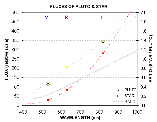
Pluto was brighter than the star at all bands (BVRI), based on
measurements made one Pluto rotation after the occultation date. Since
I observed unfiltered my effective band
was somewhere between V and R. Pluto has an unfiltered brightness
converted to R-band, CR, of 13.75,
while the star has CR = 14.60. If an R-band filter had been used a
complete occultation of the
star
should have produced a drop in brightness of 0.40 magnitude, from
a "Pluto plus star" CR = 13.35 to "Pluto only" CR = 13.75. A
centerline duration would have lasted 6.7 minutes. I was skeptical that
a
telescope as small as my 14-inch Meade could observe such a small
change with temporal resolution of 6 seconds, which corresponds to what
is needed for scientific studies of the atmosphere (the time it takes
to pass through a scale height of Pluto's atmosphere for a centerline
occultation). My exposures were 3-seconds and due to overhead for
readout, downloading and recording the image spacing was 4.8 seconds.
Here's my light curve (LC):
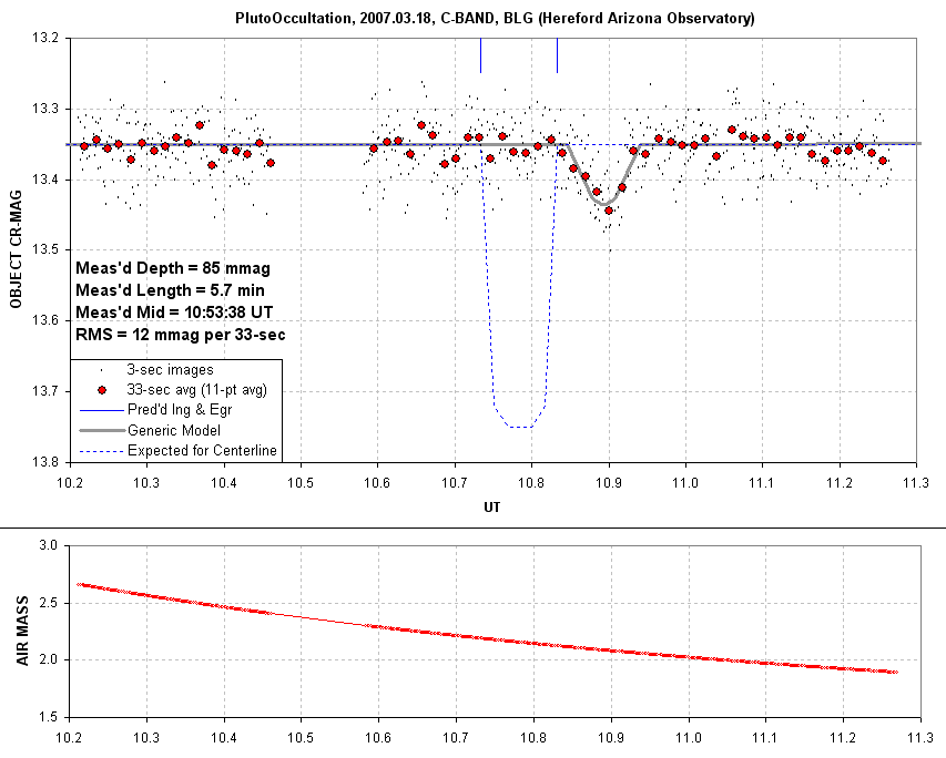
Figure 1. Light curve for a 1-hour observing session
centered on the predicted occultation. According to this presentation of the data the occultation fade has a depth
of 85 mmag, a total length of 5.7 ± 0.8 minutes (see revision below) and a mid-occultation time of
10:53:38 UT. The dashed blue trace is what was predicted for centerline
occultation (using a revised depth, based on all-sky measurements of R-magnitudes). Unfiltered, 3-second exposures
were made with a Meade LX200GPS 14-inch telescope and SBIG ST-8XE CCD.
There was no autoguiding except for an occasional manual nudge.
The maximum depth is 85 ± 10 milli-magnitude instead of the
400 milli-magnitude expected for a complete occultation of the star.
The
fade event is centered on 10:53:38 UT, or ~6.6 minutes later than
predicted. Based on the small depth
of the brightness change it is tempting to suggest that only Pluto's
atmosphere occulted the star. Observations by other observers are fit
by a model in
which the centerline was far north of my site ("off the edge of the
Earth").
There are various ways of creating a LC for the same set of
measurements. The following graph is a "folded" version that is
motivated by the expectation of symmetry about the time of
mid-occultation (suggested by Tom Kaye):
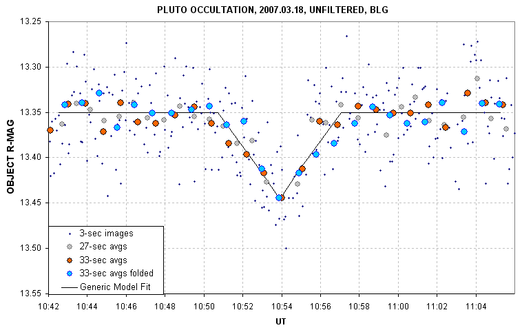
Figure 2. Zoom of the light curve's fade event. Two
averaging choices are shown (27-sec and 33-sec). The 33-sec average
data are folded about the time of minimum brightness. Depth at
mid-occultation is 96 mmag and the length (contact 1 to 4) is 6.3
minutes.
This figure may be an excessive attempt to extract information from
a noisy light curve, but for what's it worth I include it here. I've
folded
the 33-sec averaged data about the time of minimum brightness in order
to better fit a symmetrical model
for the fade event. A slight offset was adopted for the 11-point
averaging groups that produces points at the time of mid-occultation
(which might unfairly enhance the sharpness of this LC's minimum
feature). This LC's shape is better fit by
a V-shaped model. It is interesting to note that this shape argues
against a disk occultion. I
have no idea what the V-shape means. The data might just be too noisy
to attribute anything significant to the shape. With better SNR the
shape might have been seen to be flat-bottomed. Data from other
observers will be useful in sorting this out.
Another way to present same observations is to convert magnitudes to
"occulted star flux fraction" versus time. To do this it is necessary
to adopt a value for the ratio of the star's flux to Pluto's flux using
my telescope system (unfiltered). The required flux ratio is
Sstar/Spluto = 0.495, as determined on March 25 (described in a section
below this one).
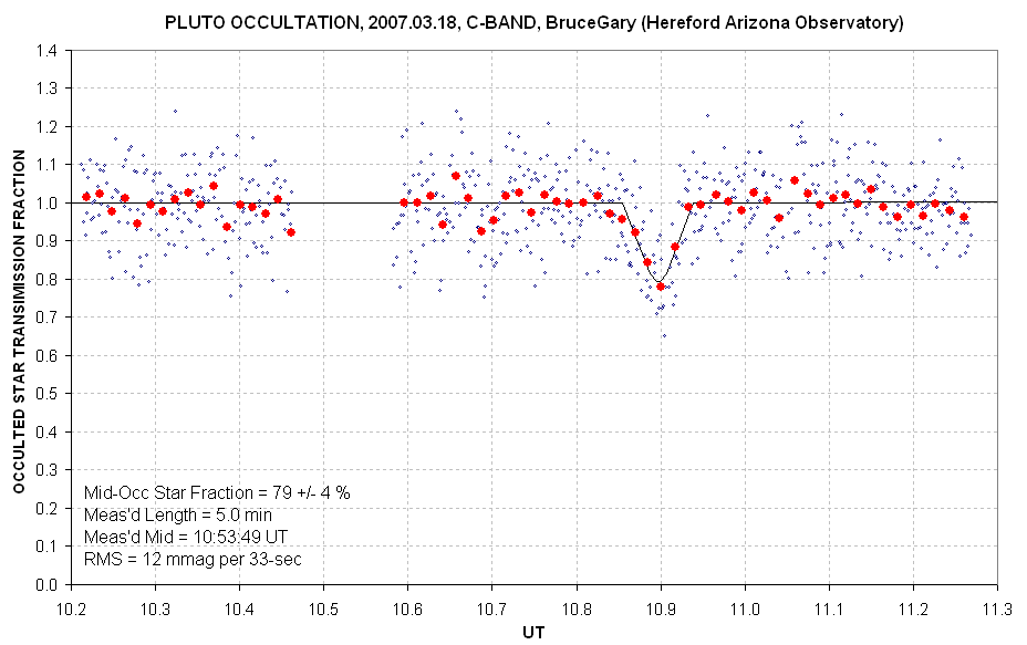
Figure 3. Star flux fraction light curve with a fit having a mid-occultation fraction = 0.79 and duration of 5.0 minutes.
Mid-occultation star flux loss = 23 ± 4 %
Total duration = 5.3 ± 0.7 minutes
The following sections present supporting observation and analyses.
My Hereford Arizona Observatory (G95) is located at Lat = +31.4522,
Lon = -110.2377 at an altitude of 4660 feet. The telescope is a 14-inch
Meade LX200GPS. My Cassegrain optics consists of a SBIG AO-7 image
stabilizer, focal reducer, CFW and SBIG ST-8XE CCD (1530x1020 pixels,
each 9 nm square). The plate scale for this configuration is 0.67
"arc/pixel. For the Pluto occultation observations I did not use the
AO-7 image stabilizer. To decrease the spacing between images I defined
a subframe of 85x62 pixels near the center of the CCD. I binned 3x3 and
recorded compressed images. The readout, downloading and recording
consumed 1.8 seconds per image, so the image spacing was 4.8 seconds. I
observed unfiltered. The CCD cooler was set to -25 C. MaxIm DL v4.58
was used to control the telescope and CCD.
At 10.45 UT I noticed the need for a focus adjustment, so I stopped
observations and used a wireless focuser to achieve ~4.5 "arc FWHM PSF
quality, and resumed observations at 10.58 UT. My polar axis is aligned
to an accuracy of about 3'arc, so there was minimal drift or image
rotation of the star field during the observations. However, on about 5
occasions I did manually nudge the telescope motors to keep the stars
as closly fixed to the pixel field as possible. The image FOV is 2.8 x
2.1 'arc, as shown in the next figure.
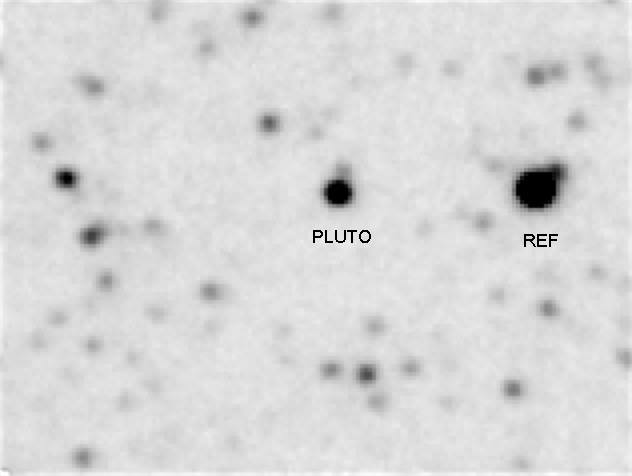
Figure 4. Finder image showing the reference star used to
monitor Pluto's brightness. The reference star is 49 "arc west of Pluto
and it is 1.9 mag brighter than "Pluto plus occulted star." The star
labeled "Pluto" is actually Pluto
plus the 14.5 mag star (so close they are on the same pixel, since this
image was made during the occultation). FOV = 2.8x2.1 'arc.
Image Processing and Data Analysis
A set of 30 dark frames were taken at the end of the
observing session, with the CCD at the same temperature as during the
occultation observations. An earlier set of darks is also available but
since the TEC cooler couldn't keep up with an ambient warming I used
only the post-occultation set of darks since they were at a more
representative temperature. The darks were taken with the same3x3
binned 85x62 subframe that was used for the occultation
observations. All raw images were calibrated using the post-occultation
master dark. No flat field correction was made. This is something I
neglected to deal with at the time, and will assess the need for making
such a flat field later.
A total of 689 images were recorded during the 1-hour
occultation session. Groups of 100 images were calibrated using the
master dark, then were offset aligned using the bright star 49 "arc to
the west. The images were doubled in size in order to accomodate an
artificial star that was added to each image (in the upper-left
corner). The artificial star has the same flux in all images, and
serves to determine extinction for the observing session. MaxIm DL's
photometry tool was used to measure fluxes for
Pluto, the reference star and the artificial star. The fluxes for these
three stars from the
group of 100 images was recorded as a CSV-file.
A program read all CSV-files and calculated air mass for
each image, then recorded a CSV-file with UT, air mass and the
magnitude differences between Pluto/star and the artificial star (used
as an intermediate reference), and the magnitude difference between the
bright star to the west (labeled "REF" in Fig. 2) and the artificial
star, for the
entire 689 image set. This file was imported to an Excel spreadsheet.
The star labeled "REF" was used to create an extinction plot (flux
versus air mass), the slope of which is identified as zenith extinction
for the observing session. For this date's observations zenith
extinction agreed with my site's typical value of 0.14
magnitude/airmass. I
adopted this zenith extinction coefficient and spreadsheet cells
calculated an
extinction corrected magnitude difference for Pluto/star and REF star.
The extinction-corrected Pluto/star magnitude was compared with the extinction-corrected REF
star magnitude to produce an offset for each image. In this way the REF
star then became the final "reference star" for the Pluto/star
measurements.Outliers were
identified using neighbor differences, and a few data were rejected
(usually just the images affected by the times I nudged the telescope
to keep the star field fixed to the pixel field). An arbitrary
magnitude offset was applied to all Pluto/star magnitudes to achieve an
average magnitude of 14.6. Eventually I'll measure the reference star's
unfiltered CV magnitude and not use the arbitrary offset.
The "model" trace in Fig. 1 is based on an exoplanet model that has
free parameters for time of ingress and egress, depth at mid-transit,
time between contact 1 and contact 2, temporal slope and an air mass
correction model (for the use of reference stars that differ in color
from the target star). For the Pluto occultation I didn't need to use
the air mass model but all other free parameters were set by hand to
produce a "pleasing fit" to the data.
Measurement of Star to Pluto Flux Ratio
The modelers need to know what fraction of the star's light was lost
during the occultation. When an asteroid occults a star the required
information is obtained by waiting an hour and imaging the same star
field. In that time the asteroid and star are far enough apart to be
measured individually. Pluto moves much slower, so waiting a day ot
more is required for that comparison image.
The professional modelers will want to know the magnitude difference
between the occulted star and Pluto, using the same telescope and
filter, and observing at the same approximate air mass. This will
enable them to convert magnitudes to star flux components, which is
needed to calculate the star's flux ratio, which I'll define as R =
Smid / So, where Smid = star flux at mid-occultation and So = star flux
out of occltation.
In case someone wants guidance converting their magnitude change to
R, the remainder of this section illustrates what's involved using my
observation as an example.
On 2007.03.25 I observed the Pluto star field with the same
unfiltered configuration used on the occultation night. The next figure
is a plot of the ratio of the occulted star's flux to Pluto's flux.
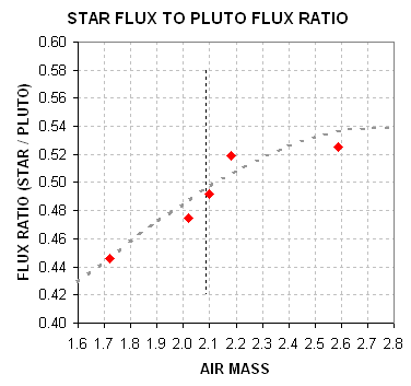
Figure 5. Ratio of occulted star flux to Pluto's flux
versus air mass, observed on 2007.03.25 when Pluto and the occulted
star were far apart. The vertical dashed line at air mass = 2.09
corresponds to the observing situation at the time of the occultation
on 2007.03.18.
The ratio of fluxes (occulted star to Pluto) is R = 0.495
± 0.015 when air mass is the same as during the occultation, m =
2.09.
This information allows us to calculate the depth of the occultation
fade in terms of only the star's flux. The star's flux component at
mid-occultation (Smid) normalized to the star's out-of-occultation flux level (Sooo),
is given by the following equation:
Smid / Sooo = ((1+R) × 2.512-dM-1)/R
Eqn 1
where R = ratio of star flux to Pluto flux (out-of-occultation),
dM = change in magnitude during occultation
For R = 0.495 ± 0.015 and dM = 0.085 ± 0.010 magnitude,
Smid / Sooo = 0.773 ± 0.027
This depth is clearly not close to zero, which suggests that the
occultation at my site was a Pluto atmospheric occultation. Based on
deeper depths at site north of mine I conclude that my light curve is a
probe of Pluto's southern polar atmosphere.
Calculating Fluxes From Magnitudes
What if an observer hasn't been able to produce a plot like Fig. 4,
but they want to make use of known magnitudes for Pluto and the
occulted star to derive a S*mid / S*o ratio?
This can be done with good accuracy provided the telescope's
"photometry coefficients" are known. These coefficients can be derived
by observing a Landolt star field and solving for the constants. For
example, my system has the following flux to Rc magnitude conversion
equation:
Rc = 19.92 - 2.5 × LOG (S / g) - 0.13 × m - 0.10 × C
Eqn 2
where S is measured star flux (using a large photometry signal aperture),
h = exposure time [seconds],
m = air mass, and
C' = C + 1.3 × C2, and C = V - R - 0.31 (note that C' is a linearized star color).
The constants and coefficients (19.92, 0.13 and -0.10) were determined by observing many Landolt stars at several air masses.
Equation 2 can be re-written:
S = g × 10 (( 19.92 - R - 0.13 × m - 0.10 × C' ) / 2.5)
Eqn 3
Each observer will have to substitute values for their telescope
system. For the purpose of this occultation task it is not necessary to
use a correct zero-shift constant (19.83 for my system), but it will be
important to know zenith extinction for your site and date, if it
changes much (0.13 mag/airmass for my site), and the star color
sensitivity coefficient is moderately important (-0.10 for my telescope
system). If BVRcIc filters are used, and if your CCD has a
QE(wavelength) function similar to mine (ST-8E with a KAF1602E chip),
then you can probably adopt my star color sensitivity coefficients:
B = +0.38 ± 0.05
V = -0.05 ± 0.03
R = -0.10 ± 0.03
I = +0.02 ± 0.03
CR = -0.20 ± 0.10
If you don't know your site's zenith extinction coefficients, then maybe the following graph can be a guide.
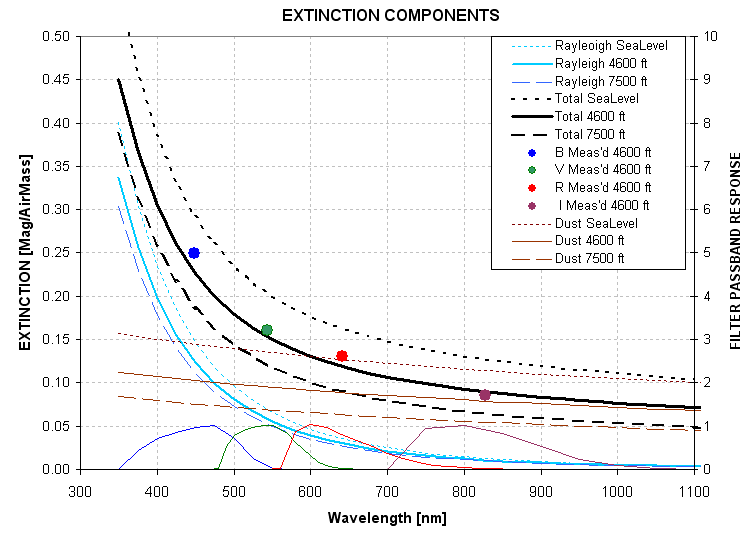
Figure 6. Extinction components (Rayleigh scattering and dust Mie scattering) versus wavelength for 3 site altitudes.
Pluto R-mag = 13.75, V-R = 0.58
Star R-mag = 14.60, V-R = 1.13
Substituting the Pluto and occulted star R-magnitudes in Eqn. 3, and
using a zenith extinction of 0.13 and star color sensitivity of -0.10,
we calculate the following fluxes for Pluto and the star:
The following false color image shows Pluto and the star it occulted.
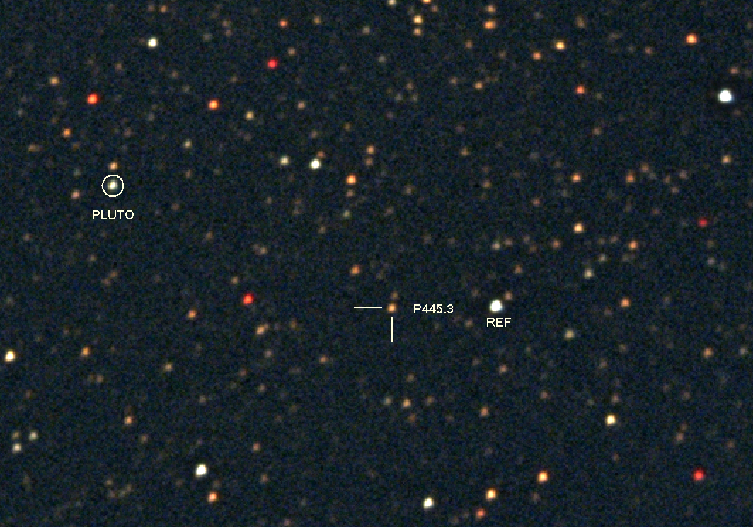
Figure 6. False color image of the Pluto occultation region on 2007.03.25 UT. In place of LRGB I used CIRV. FOV
= 11.9 x 8.3 'arc (cropped of original 17 x 1 'arc image). P445.3 is
the star Pluto occulted, and the star labeled "REF" is the one I used
for my light curve. FWHM = 3.2 "arc. [Total exposures for C, I, R and V
= 40 sec, 290 sec, 290 sec, 60 sec.]
Notice how red most stars are! This may be due to interstellar
dust reddening. After all, the galactic latitude and longitude are 3.8
and 11.6 degrees, respectively.
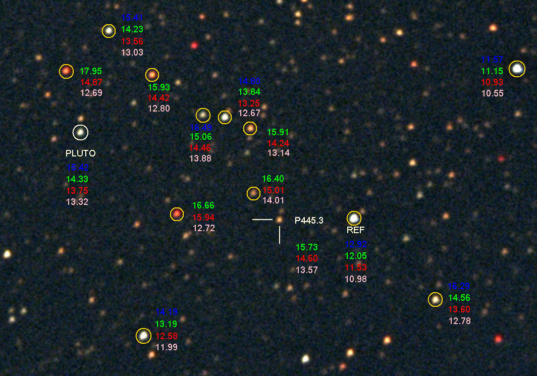
Figure 8. All-sky photometry measurements for V and Rc
magnitudes for Pluto and other stars. Since Pluto brightened 0.01
magnitude between the occultation and the time of these all-sky
calibrations, to obtain BVRcIc magnitudes for Pluto at the time
ofoccultation it is necessary to add 0.01 magnitude to the entries in
this figure. The reddest stars were too faint in B-band for useful
measurements to be obtained, and this includes the star that Pluto
occulted.
The estimated SE for V, Rc and Ic are 0.03 magnitude. This is based
on
the scatter of Landolt star magnitudes about a telescope system
coefficients solution: RMS = 0.027 mag for V (N=21), RMS = 0.017 mag
for Rc
(N = 29) and RMS = 0.026 mag for Ic (N=19). B magnitudes could not be
measured for 6 stars (the reddest stars). For those with magnitude
entries in the above figure the stochastic SE ranges from SE = 0.06 for
B = 16.5 to SE = 0.03 for B = 15.5, and is better for brighter stars.
The air mass range is 1.2 to 2.1.
Related links:
Bruno Sicardy (really neat)
Chris Peterson
Brian Warner
Tony George
Daniel Caton
Peterson, Herrero & Schlottman
Bruce's Astrophotos
____________________________________________________________________
This site opened: March 20, 2007. Last Update: April 17, 2007