This web page is a place where I summarize a procedure I use to estimate the size of an exoplanet candidate from it's transit depth and the star's color. It's so "primitive" that I am reluctant to place it in the public domain, but in case someone else is brave enough to try my procedure for estimating exoplanet size from nothing more than transit depth and star color, I shall forget caution and upload it to my server.
Suppose we know the transit depth for a possible exoplanet and we
want to assess the probability that the secondary is an exoplanet
instead of a binary star. Until Doppler information is available we
won't know the secondary's mass. But we do have information about the
primary star's "color." We might have B-V or J-K. The challenge is to
estimate the probability that the secondary is an exoplanet instead of
a small star. This web page attempts to provide a very crude answer to that question. Here's my way of
summarizing the task.
CASE STUDY
I like explaining things through the use of a specific example. The reader's job is to "generalize" the specific example.
Let's assume the following:
Transit depth = 23 ± 1 mmag,
B-V = +0.66 ± 0.05,
J-K = 0.41 ± 0.01.
There are four steps for deriving an estimate for Rp/Rj, and one
additional step for assessing whether this indicates a planet or a
brown dwarf. Caveats for all of this are given at the end.
1) Getting Spectral Class
The following graphs provide a means for estimating the star's spectral classification, SC.
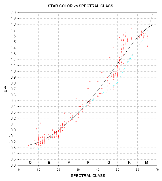
Figure 1. Star color B-V versus spectral classification.
Diamonds are from a table of 314 stars brighter than 3.55
(http://www.astro.utoronto.ca/~garrison/oh.html). The two dashed traces
are from Lang (1992) and a table on a web page
(http://cosmos.phy.tufts.edu/~zirbel/laboratories/Photo1.pdf#search=%22Star%20B-V%20spectral%20class%22).
Using Fig. 1 to convert B-V = 0.66 ± 0.05 to SC yields the result SC = G0 (using the 314 bright star plot) or SC = G4 (using the two traces). I don't know "the story" behind the big discrepancy for G and cooler stars, so in this case I'll adopt the average and say that SC = G2± 3.
We can also use the J-K star color to derive SC.
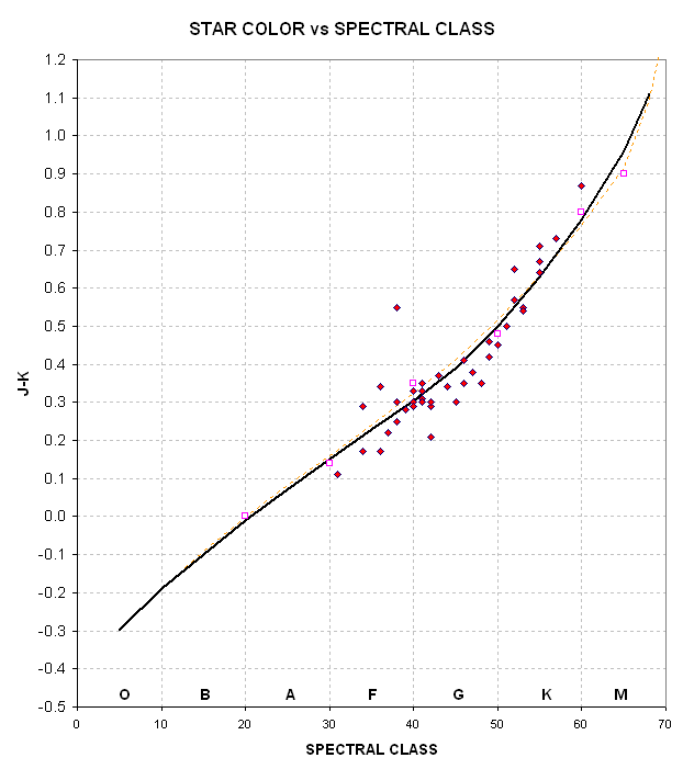
Figure 2. Star color J-K versus spectral classification.
Plot is based on graphs found on web
(http://www-int.stsci.edu/~inr/intrins.html)
Using Fig. 2 to convert J-K = 0.41 ± 0.01 to SC yields the result SC = G5 ± 5.
This SC result is compatible with the SC derived using B-V. Which is better?
Hot stars exhibit a greater variation of B-V than J-K, whereas cool
star are the opposite. The next graph shows how poor SC solutions are
for hot stars when they are based on J-K.
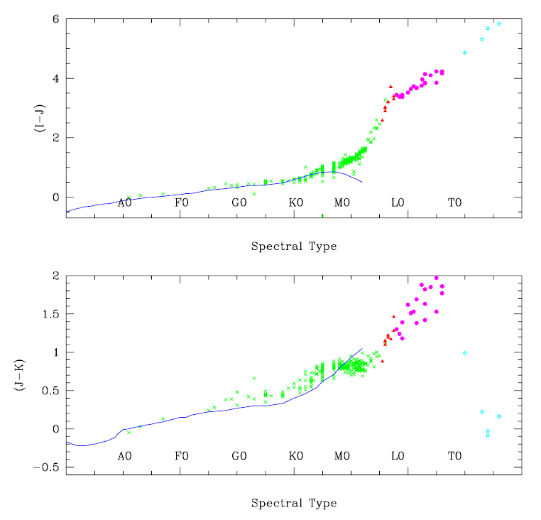
Figure 3. 2MASS colors versus spectral classification. From web site (lost URL).
Notice that for stars hotter than ~K0 there isn't much of a change
to J-K versus spectral class. The opposite is true for B-V. This is due
to the shape of the blackbody spectrum shifting with surface
temperature; for cool stars B-V is the same because the B and V filters
are on the blue side of the peak, whereas for hot stars J-K is the same
because both J and K are on the red side of the peak.
Whenever information for both colors is available it is a good idea
to derive SC with an associated uncertainty using both Fig's 1 and 2.
I conclude the SC assignment by combining the two estimates: SC = G2 ± 3 and G5 ± 5:
SC = G3 ± 3
2) Converting SC to Rstar
The next figure shows how Rstar varies with SC.
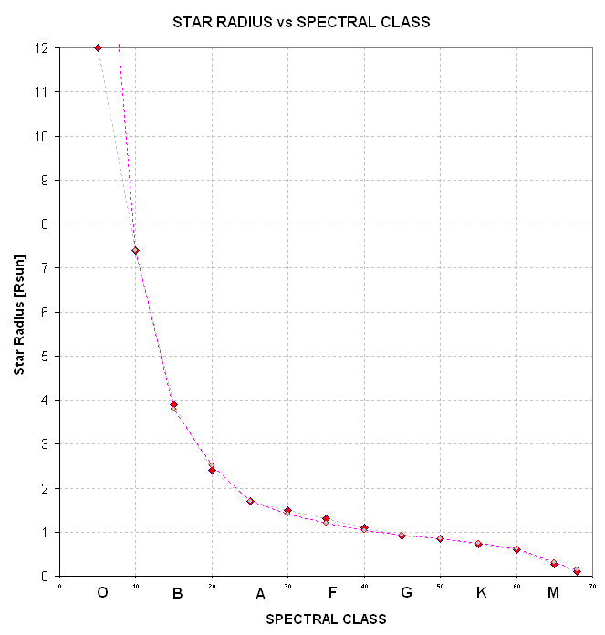
Figure 4. Star radius versus spectral class, SC.
And here's a version with an expanded star radius scale.
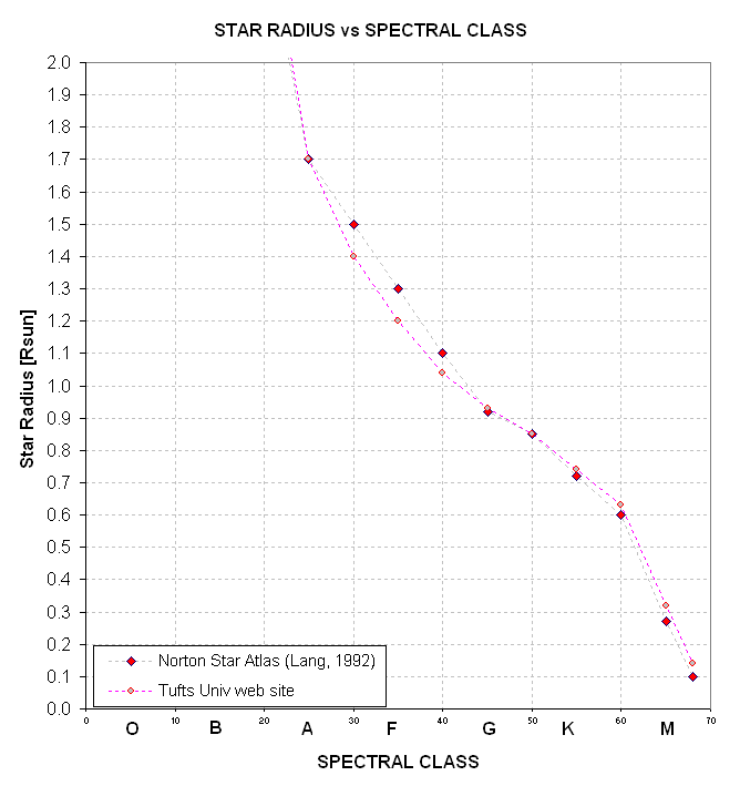
Figure 5. Star radius versus spectral class, SC.
If SC = G3 ± 3 then Rstar/Rsun = 0.97 ± 0.07.
3) Getting Rp/Rstar
The transit depth for this case study is 23 ± 1 mmag. If the
planet, or secondary star, crosses the primary (which we assume is
larger than the secondary) in such a way that all of the secondary is
within the solid angle of the primary, the geometry is
straight-forward. Transit depth can be calculated from
Transit Depth [mmag] = -2500 LOG 10 (1 - Rp/Rstar )
<>This equations assumes two things: 1) the planet's solid angle has a circular shape, and 2) the star is uniformly bright (no limb darkening). We'll have to accept the first assumption, but the secnd one can be modeled. A typical star's limb darkening varies with distance from center in the following way:| r / Rstar |
B / Bavg |
| 0.00 |
1.01 |
| 0.50 |
0.95 |
| 0.75 |
0.86 |
| 0.90 |
0.68 |
In this table Bavg is the disk average brightness.
The following graph shows
![]()
Figure 6. Transit depth [mmag] versus planet's size
relative to the star. The 4 traces correspond to transits with a
closest approach going through the star's center (top trace) to missing
the center by 0.90 star radii (bottom trace).
The next graph emphasizes the region of interest for interesting transits.
![]()
Figure 7. Transit depth [mmag] versus planet's size relative to the star. The 4 traces correspond to transits with a closest approach going through the star's center (top trace) to missing the center by 0.90 star radii (bottom trace).
For our case study, with transit depth = 23 ± 1 mmag, a
transit path that goes through the star's center corresponds to a
planet size of Rp / Rstar = 0.14 ± 0.01.
A more likely scenario is for the transit closest approach to be ~0.40
Rstar. Why 0.40? If closest approach were 1.00 only half the planet's
solid angle would produce a transit, and it would be very brief. Such a
transit is not likely to be detected, so it wouldn't show up as a
candidate. A closest approach of ~ 0.80 would produce a nearly full
amplitude transit. Everything between ~ 0.00 and 0.80 can be considered
both suitable for becoming candidates and equally likely. It is better
to adopt a closest approach of 0.40 assumption in the absence of
information to argue for a different geometry. Therefore, we convert
the 23 ± 1 mmag transit depth to
Rp / Rstar = 0.145 ± 0.025/0.005
4) Getting Rp/Rj
It is now a simple matter to convert the previous solutions to
arrive at a planet size in terms of Jupiter's equatorial radius. Note,
Jupiter's equatorial radius is 6.4% greater than its polar radius, so
its solid angle is ~3.2 % less than a circle with radius Rj. However,
the exoplanet community has carelessly adopted Rj = 71492 km, Jupiter's
equatorial radius, and exoplanet sizes are given as if Jupiter has a
circular shape with that radius.
Our sun's radius is 9.73 times larger than Jupiter's equatorial radius. So,
Rp/Rj = 9.73 * Rp/Rstar *
Rstar/Rsun
Eqn. 1
Rp/Rj = 1.37 ± 0.26 / 0.11
The greatest source of uncertainty is not knowing the planet's
closest approach distance. This can be determined from the shape of the
transit, but we're not dealing with a complete solution on this web
page.
5) Probability of Planet vs. Brown Dwarf
With a planet size we now face the question "Is it a planet or a
brown dwarf?" If we knew its mass (from Doppler measurements) we could
settle that question. But on this web page we're limited to knowing
only the transit depth and star color. The smallest brown dwarf known
has Rstar/Rsun ~1.2. I don't think we know how common this is, but
eventually we may know that. What we want is a graph of the probability
that an object with a known size is either a planet or a star. For
example, consider the following estimate.
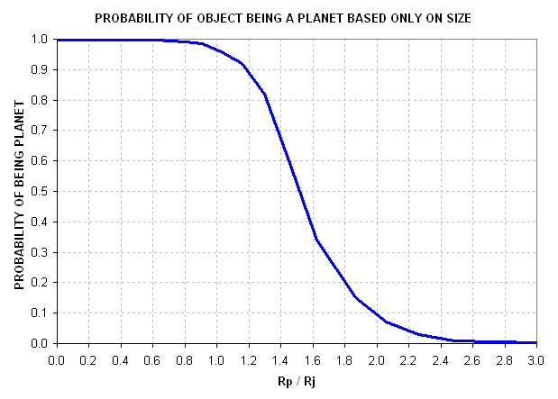
Figure 8. Probability of an object's being a planet instead of a star based only on its size (just my guess).
If this graph is adopted then an object with Rp/Rj = 1.37 has a high probablity of being a planet.
This is the end of our case study example. Consider the question posed by the next section.
HOW REASONABLE ARE THE RESULTS OF SUCH A PROCEDURE?
The case study considered above (transit depth = 23 mmag, B-V =
+0.66, J-K = +0.41) is not a hypothetical example with values chosen at
random. It describes exoplanet XO-1b. We can now evaluate how well the
simple procedure I've described compares with a detailed analysis of
the transit shape, star's spectral type based on high-resolution
spectra, and Doppler observations used to establish the planet's mass.
There are two published studies giving a planet size (McCullough et al,
2006, and Wilson et al, 2006). I'll present the 3 solutions for planet
size in the next table.
| Source |
Rp / Rj |
| My simple procedure |
1.37 ± 0.26,0.11 |
| McCullough et al |
1.30 ± 0.11 |
| Wilson et al |
1.34 ± 0.12 |
This analysis assumes that the primary star is on the main sequence.
That's a 90% good assumption. It might even be better than 90% if you
consider the fact that we're only dealing with stars having a nearby
companion, either a planet or small star, which may not survive the
ravages of stellar swelling and brightening that accompanies some
departures from the main branch.
There seem to be more eclipsing binaries than transiting exoplanets.
Therefore, when transit shape is ignored and the only information we
have is that depth = 60 mmg, for example, it may be more likely that
such a transit depth is produced by a grazing eclipse by a binary star
than by a full transit (all of the planet's solid angle covering part
of the star) by an exoplanet.
Another possibility when only transit depth is known is that there
are two stars within the photometry aperture and the fainter of the two
is an eclipsing binary with a large depth.
In both cases a detailed transit shape should help identify whether or not an exoplanet is likely. A "flat bottom" would favor an exoplanet.
____________________________________________________________________
This site opened: August 21, 2006. Last Update: September 03, 2006