INTRODUCTIONBruce L. Gary; 2007.03.04, updated 2010.10.22This web page is a place where I summarize a procedure I use to estimate the size of an exoplanet candidate from the transiting star's spectral class, transit depth, transit length, orbital period and filter band. A link is included for downloading an Excel spreadsheet that performs the calculations.
A proper solution for planet radius from a LC will involve more information about the LC's shape than is used by the simple solution on this page. A crude method is presented for determining if the shape is similar to what an exoplanet can produce, versus what a blend of an eclipsing binary (EB) with another nearby star would produce. My shortcuts reduce accuracy, of course, but if an approximate answer is acceptable then the procedures described here may be useful.
I like explaining things through the use of a specific example. The reader's
job is to "generalize" from the specific. I'm going to treat real observations
of a "mystery" star's transit light curve; this way we can grade the results
of my crude analysis procedure using a rigorous treatment by professionals.
Let's assume the following:
which were derived from the following transit light curve (measured with
an amateur 14-inch telescope).
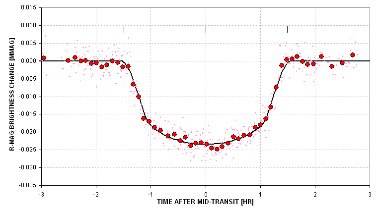
Figure 1.01 Transit light curve for a mystery star whose LC
we shall try to "solve" using the procedures described on this web page.
After a transiting candidate has been observed, and before radial velocity
measurements have been made to assess the mass of the secondary, this is
all the information we have to work with. Using this limited information
there are many steps for interpreting the LC to estimate secondary size,
Rp/Rj.
At this point we have an approximate planet size. It's a first iteration
since limb darkening has been neglected. The next group of operations is
a 2nd iteration.
Star's mass, Mstr = 0.97 (times sun's mass)No more iterations are needed since the two miss distance results (& limb darkening corrections) are the same. We have a stable solution:
Mstr = 2.57 - 3.782 * (B-V) + 2.356 * (B-V)^2 - 0.461 * (B-V)^3
Planet orbital radius, a = 7.22e6 [km]
a = 1.496e8 * [Mstr^1/3 * (P / 365.25)^2/3], where P[days], Mstr[sun's mass] & a[km]
Transit length maximum, Lx = 3.28 [hr] (corresponds to central transit)
Lx = 2 (Rstr * Rsun + Rp/Rj * Rj) / (2 pi a / 24 * P) where Rsun = 6.955e5 km, Rj = 7.1492e4 km
Miss distance (also called "impact parameter"), b = 0.42 (ratio of closest approach to center divided by star's radius)
b = SQRT [1 - (L / Lx)^2]
Limb darkening effect, LDe = 1.16 (divide D by this)
I(b)/I(av) = [1 - 0.98 + 0.15 + 0.98*c - 0.15*c^2] / 0.746, for B-band
" = [1 - 0.92 + 0.19 + 0.92*c - 0.19*c^2] / 0.787, for V-band
" = [1 - 0.85 + 0.23 + 0.85*c - 0.23*c^2] / 0.828, for R-band
" = [1 - 0.78 + 0.27 + 0.78*c - 0.27*c^2] / 0.869, for I-band
where c = SQRT(1 - b^2) (= cosine(theta), and theta is angle between line-of-sight and star radius line to location of nearest approach of exoplanet to star center)
- Corrected transit depth, D = 20.4 mmag (1st iteration for D)
- D = D / LDe (this is the D that would have been measured if the star were uniformly bright)
- Planet radius, Rp/Rj = 1.31 (2nd iteration for Rp/Rj)
- (Same eqn as above but now assumes b = 0.42 and appropriate limb darkening)
- Transit length maximum, Lx = 3.25 [hr] (2nd iteration for central transit length)
- (Same eqn as above)
- Miss distance, b = 0.405
- (Same eqn as above)
- Limb darkening correction, LDe = 1.165 (divide D by this)
- (Same eqn as above)
Rp/Rj = 1.306
To assign a SE to this solution it is necessary to repeat the above procedure
using a range of values for the measured transit depth and length. When this
is done (using the Excel spreadsheet, below) we get Rp/Rj = 1.306 +/- 0.063
(with B-V uncertainty contributing the greatest component of SE). Note that
the stated SE doesn't include the uncertainties associated with the equations
converting B-V to stellar radius and mass, nor does it allow for the possibility
that the star is "off the main sequence.".
The B-band light curve for XO-1 is measured to have D = 24.8 ±
0.5 and L = 2.95 ± 0.03. For these inputs the procedure described
above gives Rp/Rj = 1.29 +/- 0.06.
GRAPHICAL REPRESENTATION OF EQUATIONS
The following graphs can be used instead of the equations for deriving
star radius, mass and limb darkening correction (derived from Allen's
Astrophysical Quantities, Fourth Edition, 2000):
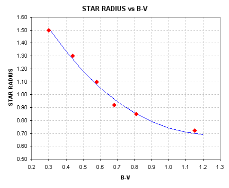
Figure 1.2. Converting star color B-V to stellar radius (assuming main sequence).
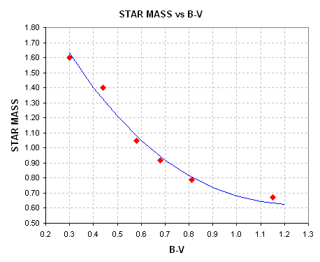
Figure 1.03. Converting star color B-V to stellar mass (assuming
main sequence).
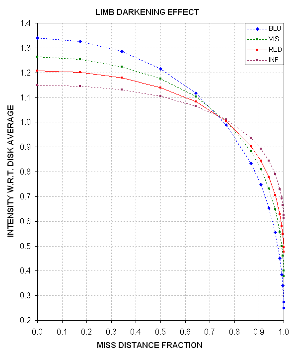
Figure 1.04. Converting miss distance ("b") and filter band to intensity at that location, normalized by disk-average intensity (assuming a sun-like star).
The following two figures show how transit shape depths chould behave
when the miss distance changes from near-center to near-edge. These are real
measurements (graciosly provided by Cindy Foote) that were categorized as
EB based on the depth values. The concept is the same, whether it's an exoplanet
or small EB, because in both cases a central transit produces a greater loss
of light in B-band than R-band, and for a near-edge transit the reverse is
true.
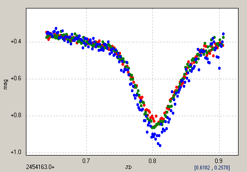
Figure 1.05. Transit depth is greatest for B-band, consistent
with miss distance b < 0.73 (coutesy of Cindy Foote, 2007.03.04).
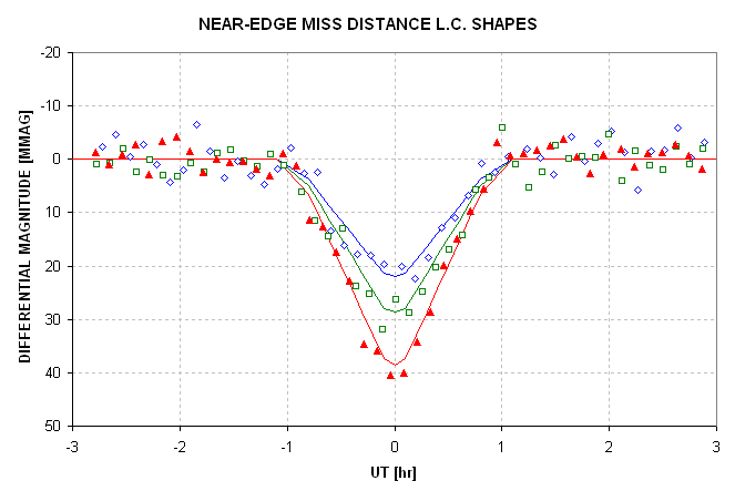
Figure 1.06. Transit depth is greatest for R-band, consistent
with miss distance b > 0.73 (coutesy of Cindy Foote, 2007.03.04).
2.0 VERIFYING THAT LIGHT CURVE SHAPE
IS NOT AN E.B. BLENDING
Wide-field survey telescopes provide an efficient means for detecting
stars that are undergoing periodic fadings with depths small enough to be
caused by an exoplanet transit. A fundamental limitation of such a survey
is that in order to achieve a wide field of view the telescope's resolution
is poor, and this leads to many "false alarms" due to the "blending" of light
from stars within the resolution circle. If, for example, the resolution
circle has a radius of 1 'arc and the star flux within this circle corresponds
to ~11th magnitude, it is common for several stars to be present within the
resolution circle that are fainter than 11th magnitude but with fluxes that
add up to 11th magnitude. If this situation occurs, and when one of those
stars is an eclipsing binary (EB) with a large transit depth, the transit
depth measured by the survey telescope may be small enough to resemble one
produced by a planet. This is a common occurence.
There are two blending situations that need to be considered: 1) the EB
is part of a triple star system, so the blending star is too close to the
EB to be resolved by even large telescopes, and 2) the EB and the blending
star are far enough apart (usually gravitationally unrelated but close together
in our line-of-sight) that their angular separation are within the resolution
limits of ground-based telescopes. The second of these blending situations
is probably more common than the first.
When a survey telescope system produces many candidates per month it is
not feasible to rule out an EB explanation for each one by measuring radial
velocities during the course of a few nights with a telescope large enough
to produce spectrograms that have the required accuracy. Although radial
velocity measurements would allow the determination of the secondary's mass,
and thus distinguish between EB and planet transits, large telescope time
is too costly for such an approach unless there is good evidence ruling out
an EB explanation and leaving open the exoplanet possibility.
A better alternative is to perform follow-up observations of the survey
candidates using telescope's with apertures sufficient to identify the most
common blending situation. Amateurs with 14-inch aperture telescopes, for
example, have sufficient resolution to determine which star within the survey's
resolution area is undergoing transit, thus easily identifying most cases
of non-gravitationally related blending. These telescopes also have sufficient
SNR for an 11th magnitude star, for example, to allow the transit light curve
to be determined with good enough quality to sometimes identify the presence
of a triple star system EB. There may be many more cases of triple star EBs
that resemble exoplanet transits than there are actual exoplanet transits.
Therefore, it is important to be able to interpret a transit light curve
to distinguish between a triple star EB and an exoplanet.
This section demonstrates how amateurs can distinguish between exoplanet
light curves and "EB triple star blended light curves" of similar depth,
so that additional amateur observing time is not wasted on non-exoplanet
candidates.
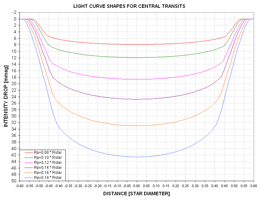
Figure 2.01. Model light curves for central transits by different
sized secondaries. An R-band sun-like limb darkening function was used.
First contact occurs when the intensity begins to drop, and second contact
can be identified by the inflection where the slope changes from steep to
shallow. A "shape" parameter is defined as the ratio of time the secondary
is partially covering the star to the entire length of the transit (e.g.,
contact 1 to contact 2 divided by contact 1 to mid-transit). For example,
in the above figure consider Rp/Rstr = 0.12: contact 1 and 2 occur at -0.55
and -0.44, and contact 1 to mid-transit is 0.55. For this transit the shape
parameter is S = (0.55-0.44) / 0.55 = 0.20.
Let's estimate the shape parameter for a real transit.
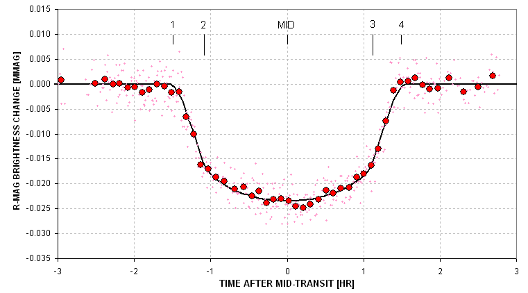
Figure 2.02. Measured light curve with the contact times indicated.
My readings of contact 1 and 2 are -1.48 and -1.05 hour. The shape parameter
is therefore 0.29 (0.43 / 1.48). Assigning SE uncertainties and propogating
them yields: S = 0.29 ± 0.01.
The following figure shows how the shape parameter varies with secondary
size for central transits.
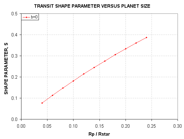
Figure 2.03. Shape parameter, S, versus planet size for
central transits.
We next consider how the LC shapes vary with miss distance. We'll adopt
one secondary size and vary the miss distance.
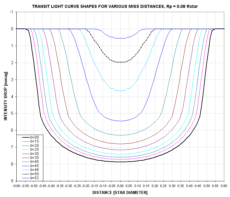
Figure 2.04. Shape of LCs for various miss distances (b)
and a fixed secondary size of Rp/Rstr = 0.08.
Note the change of terminology for "center miss distance" from m
to b. Sorry, but I use both symbols for this parameter throughout
this web page.
The following figure summarizes the dependence of S on many choices
for planet size and miss distance.
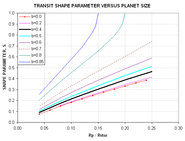
Figure 2.05. Shape parameter for a selection of secondary sizes
and center miss distances, b.
Recall that for this LC we determined that S = 0.29 ± 0.01.
The shape alone tells us that Rp/Rstr < 0.17. From the previous section
we derived m = b = 0.40 (the thick black trace in the above
figure), so this means Rp/Rstr ~ 0.13. It's not our purpose here to re-derive
Rp/Rj, but let's do it to verify consistency. Rp/Rj = 9.73 * Rp/Rstr * Rstr/Rsun
= 9.73 * 0.13 * 0.99 = 1.25. This is smaller than 1.31 derived from the transit
depth, but notice that the 1.25 estimate came from the light curve shape,
S, and extra information about miss distance. This consistency check
is successful.
Our goal in this section is merely to distinguish between exoplanet light
curve shapes and EB shapes. It will be instructive to consider secondaries
at the threshold of being a star versus a planet. This is generally taken
to be Rp/Rj ~1.5. For such "threshold secondaries" the Rp/Rstr will depend
on the size of the star, which in turn depends on its B-V (spectral type).
Let's list some examples, going from blue to red stars.
Blue star (B-V ~ 0.30, spectral type F1V), Rstr/Rsun
~1.5, Rp/Rstr ~0.10
Sun-like (B-V ~ 0.65, spectral type G2V), Rstr/Rsun ~1.0,
Rp/Rstr ~0.15
Red star (B-V ~ 1.20, spectral type K6V), Rstr/Rsun ~0.7,
Rp/Rstr ~0.22
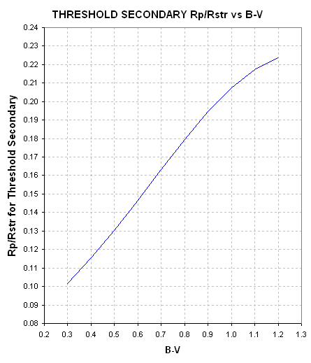
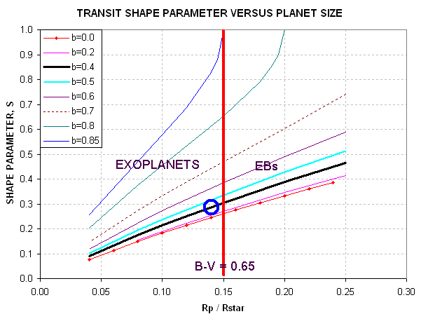
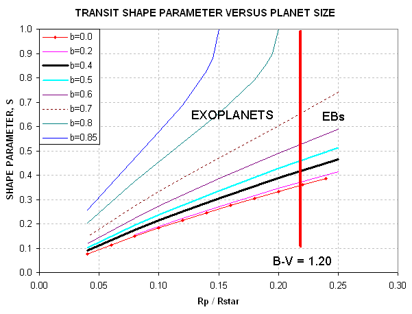
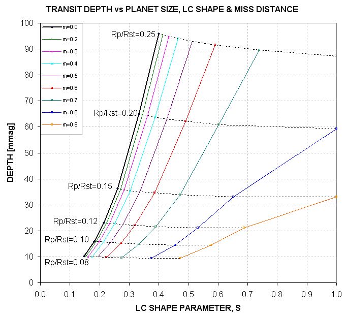
Figure 2.08. Domains for exoplanets and EBs, using parameters S and D as input (yielding Rp/Rstr and miss distance as answers).
This figure requires knowledge of transit depth, D, instead of
miss distance. This is better since D is easily determined by casual
inspection of a LC. The shape parameter S is also easily determined
by visual inspection. Therefore, without any attempts to "solve" the LC this
plot can be used to estimate Rp/Rstr and miss distance. Then, by knowing
B-V we can specify a Rp/Rstr "threshold secondary" boundary in the figure
that separates the exoplanet and the EB domains.
Consider the previous example, where XO-1 was determined to have S
= 0.29 and D ~ 24 mmag. Given that B-V = 0.66 we know that a
"threshold secondary" will have Rp/Rstr = 0.156 (cf. Fig. 2.6). Now, using
the above figure draw a trace at this Rp/Rstr value, as in the following
figure.
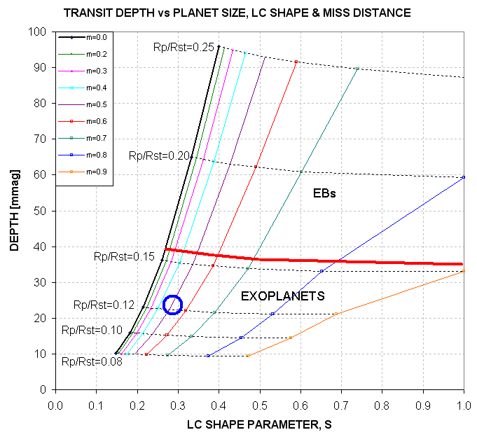
Figure 2.09. Domains for exoplanets and EBs for independent
variables S and D with a "threshold secondary" Rp/Rstr domain
separater (thick red trace) at Rp/Rstr = 0.16, corresponding to B-V = 0.66.
The blue circle corresponds to the S and D location for XO-1.
From this graph it is immediately apparent that, subject to the assumptions
of the model, XO-1 is an exoplanet instead of an EB. This conclusion does
not require solving the LC for Rp/Rstr, as described in Section 1. Indeed,
this graph gives an approximate solution for miss distance, m = 0.5 (not
as accurate as the solution in Section 1, but somewhat useful).
Here's a handy plot showing "threshold secondary" boundaries for other
B-V values.
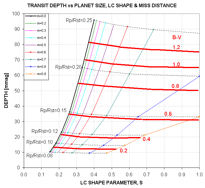
Figure 2.10. The thick red traces are "secondary threshold"
boundaries, labeled with the B-V color of the star, above which is the EB
realm and below which is the exoplanet realm.
Now that you understand the concepts I can save you time by offereing
an Excel spreadsheet that does most of what's described on this web page.
The user simply enters LC depth D, LC length L, and star color B-V in the
appropiate cells and the spreadsheet calculates a 3-iteration solution for
Rp/Rj (provided a solution exists). Here's the link for the Excel spreadsheet
that does everything described in Section 1: RpIterationExcelSpreadsheet
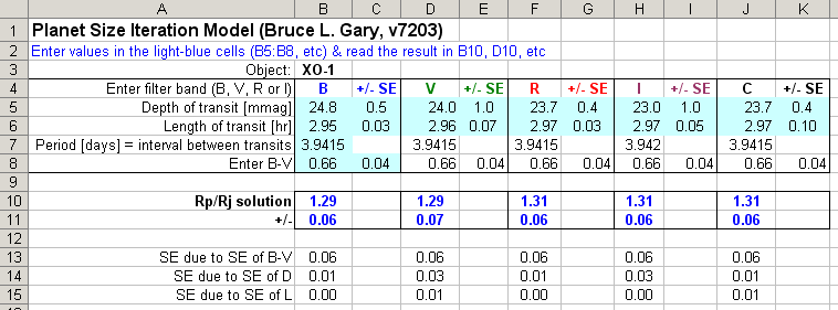
Figure 4.01. Example of the Excel spreadsheet with XO-1 entries
for several filter bands (B5:C8 for B-band, etc) and the Rp/Rj solution (B10:B11
for B, etc).
The line for SE of "Rp/Rj solution" is based on changes in D, L and B-V
using their respective SE. In this example note that the Rp/Rj solutions
for all bands are about the same, 1.30. This provides a good "reality check"
on data quality as well as the limb darkening model. Rows 13-15 show the
SE on Rp/Rj due to the SE on B-V, D and L separately. The largest component
of uncertainty comes from B-V. Even if B-V were known exactly there's an
uncertainty in converting it to star radius and mass, given that the "main
sequence" of the HR diagram consists of a spread of star locations and there's
a corresponding spread in the relationship bewteen radius versus B-V and
mass versus B-V.
A future version of this spreadsheet will include a section for the user
to enter a transit shape parameter value, S, and an answer cell will
show the likelihood of S/D being associated with an exoplanet versus an EB.
I also plan on expanding the limb darkening model to take into account limb
darkening dependence on star color.
____________________________________________________________________
This site opened: March 3, 2007 Last Update: 2010.10.22