The "statistical retrieval" (SR) procedure is a favorite method for converting remotely-sensed observables to desired physical properties, called "retrievables." It is an all-purpose tool that has found applications in many fields besides remote sensing. The same factors that render it powerful also render it dangerous on occasion. It must be used carefully, with awareness of limitations and pitfalls. Since each situation can usually be served by many possible retrieval procedures, it is important that these strengths and weaknesses be "kept in mind" in relation to the intended use. Sometimes the SR procedure may not offer the best match to the user's needs. This sub-section will briefly sketch how the procedure works, and highlight its main strengths and weaknesses.

It will be useful to think in terms of "reality space" and "observable space." In reality space are the things we want to have values for, such as air temperature at a specific altitude. In observable space are the things our instruments measure, such as brightness temperature at a specific frequency and viewing direction. Both "spaces" can have any number of dimensions. It is straightforward to calculate where in observable space a set of measurements should be if we first specify the reality space location. This assumes, of course, that we have complete knowledge of the physics governing thermal emission and intervening absorption and scattering. There are no ambiguities transforming in this direction. For every hypothesized location in reality space our physical model "maps us over" to only one location in observable space, as illustrated by situations A, B and C in Fig. 10.1 (note that realities B and C map to the same location in observable space).



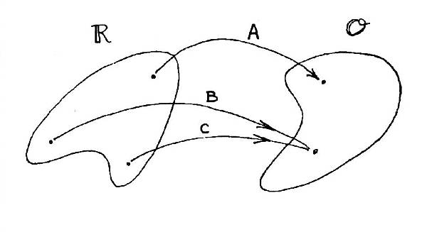
Figure 10.1 Mapping forward from Reality Space to Observable Space.



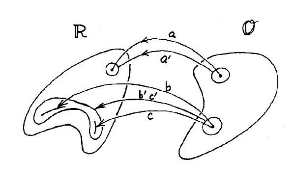
Figure 10.2. Mapping backwards from Observational Space to Reality Space.

It is not straightforward "mapping back," going from observable space to reality space. Indeed, there are ambiguities; one location in observable space may map over to many points in reality space, as illustrated by situations "b" and "c" in Fig. 10.2. This situation can occur when observables are integrated quantities, like brightness temperature. When observing uncertainties are taken into account we are dealing with mapping back from areas in observable space to areas in reality space, as shown by a' in Fig. 10.2. For the situation in which more than one reality produces identical (or nearly identical) observables a small area in observable space can map back to a large area in reality space. This is depicted in Fig. 10.2 as situation b'c'. 
  <>
These examples illustrate how care must be taken in transforming observables to an inferred reality. It is necessary to assure that the "best" solution is obtained, and to assure that formal uncertainties take proper account of the mapping ambiguities. Sometimes the "best" solution is one that is known to occur often in reality, even though its corresponding observables are no better than those corresponding to some alternative reality. The SR procedure can be used to do a powerfully good job of this.

It is true that the SR procedure unfairly favors the more likely retrieval. Thjis can be viewed as a strength of the SR method. However, there are situations when the this is a weakness. It sometimes happens that a specific and unusual meteorological siituation is to be studied. For example, the winter polar vortex can be very cold at high altitudes, giving the appearance of a very high second tropopuase. This T(z) shape will not appear in the archive of old RAOBs, before CFC mixing ratio had become as large as it is today. Moreover, polar vortex T(z) shapes are under-represented in the RAOB archive because there are fewer RAOB stations at polar latitudes. And in addition, RAOB baloons tend to burst when they are very cold, and lose their elasticity, so this further reduces the cases of cold T(z) RAOBs in the archive. When the MTP user anticipates a situation for which the RAOB archive is unlikely to favor the T(z) shape that is to be studied there are at least a couple alternative strategies. First, it may be advisable to conjure up "fake" T(z) shapes designed to represent those that are to be studied, and treat them as if they were from RAOBs by adding them to the mix with actual RAOB T(z) data. Second, the user could rely upon the original Backus-Gilbert retrieval method. The B-G retrieval makes no assumptions about which T(z) shapes are more likely to be encountered, so the unusual shapes are therefore given a fairer chance of being retrieved compared to the SR retrieval method.<>
<>
The SR procedure consists of two parts. First an archive is created, consisting of paired sets of realities and observables. For example, we might begin with 100 radiosondes. For each radiosonde we note the values of the parameters we want to retrieve and we calculate what the observable values should be (using a good physical model and a perfect measuring instrument). This will produce 100 sets of observable locations paired with their corresponding reality locations. (The use of the term "location" is merely a shorthand way of referring to a set of values, corresponding to a "vector" in either observable or reality "space.") In the example just cited, the observables are "simulated" using a believable physical model.

It is also possible to use real measurements in the SR analysis, perhaps taken specifically for creating an SR archive. Using real observables instead of caclulated ones is a an uncommonly used variant, yet it has the advantage of being unaffected by shortcomings of the physical model for emission and it also allows for calibration systematic errors in a way that will not adversely affect later retrievals. This desireable feature of using real measurements instead of calculated ones means that if the MTP instrument changes (if it's repaired, or improved in some way) its measurements may have different systematic errors which will invalidate the use of the retrieval coefficients derived from its earlier use.

The next chapter treats MTP observing strategy tradeoffs between angle-scanning and frequency sampling. The user of an existing MTP won't benefit by that discussion, but anyone designing an MTP will want to understand the relative merits of these two observing philosophies.


Go to next Chapter #11
Go to previous Chapter #9
Return to Introduction

____________________________________________________________________

This site opened:  October 16, 2005.  Last Update:  June 22, 2007