This web page presents some of the floundering this amateur underwent while attempting to derive an all-sky photometry solution for the star field centered on HD 37605 (hereafter referred to as E0540).

2004 Dec 10 All-Sky Observations

First Photometric Group

I will use the term "photometric group" to refer to an observing sequence that achieve an approximately equal air mass (m) for observations of both the Landolt Area (LA) and the unknown star field, or Region of Interest (ROI). A photometric group consists of BVRI images for the LA and BVRI images for the ROI. There are a total of 8 images that must be measured, 4 for the LA and 4 for the ROI. Each of these 8 images is obtained by median combining 10 frames that have been calibrated (raw frame that has been dark subtracted and flat field corrected).

On 2004.12.10 I performed two "photometric group" observations, one at m = 2.4 and the other at m = 1.8.  Each photometric group produces a complete all-sky photometry solution for the ROI. This section describes my attempt to achieve an all-sky photometric solution from the first photometric group.

The first step in my procedure for producing an all-sky photometric sequence is to solve for one unknown term in an equation for magnitude as a function of star intensity, exposure time, air mass and star B-V color. This is done using the Landolt stars, with known magnitudes (and colors). For this first photometric group I obtained the following equations:



Figure 1. Equation magnitudes that account for measured intensity (INT) for Landolt stars, using their known magnitudes, B-V colors, air mass (m) and exposure time (g) for BVRI filter observations. Other more extensive observations have produced values for the coefficients related to extinction, star color and the product of air mass and star color; only the first term, a constant, is solved for using the Landolt stars.

When these magnitude equations are applied to the Landolt star measure intensities they yield a set of magnitudes that can be compared with the true magnitudes, shown in the next figure.

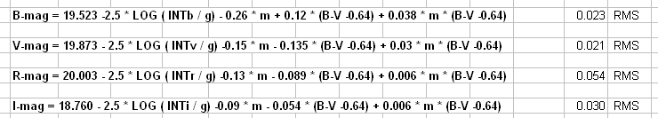
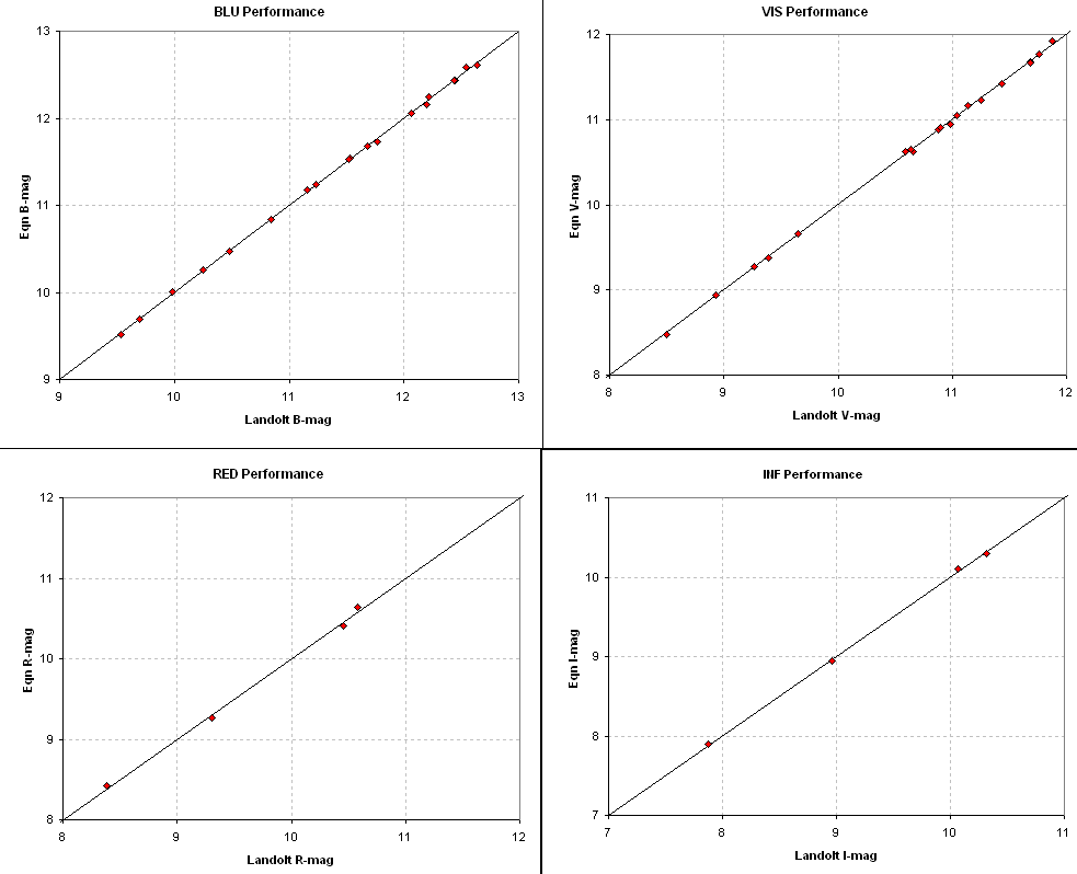
Figure 2. Comparison of equation magnitude solutions with Landolt magnitudes for the LA0540 (Landaolt Area at RA = 05:40, Dec ~0). RMS scatter is 0.023, 0.021, 0.054 and 0.030 magnitude (for B, V R and I). Observations were made on 2004.12.10 at an air mass of ~1.8. 

These 4 panels show that the equation magnitudes can produce acceptable fits with typical SE of ~0.03 mag by adjusting only one constant (zero offset) in each filter's equation relating B-V, air mass, exposure time and measured intensity.  The next set of 3 graphs were produced by comparing colors for the unknown star field (E0540) using the magnitude equations and constant solutions. If the 4 constants that work for the Landolt fields also work for the unknown star fields, then the color/color scatter diagrams for the unsknown stars should be in approximate agreement with the corresponding color/color scatter diagrams for the landolt stars.

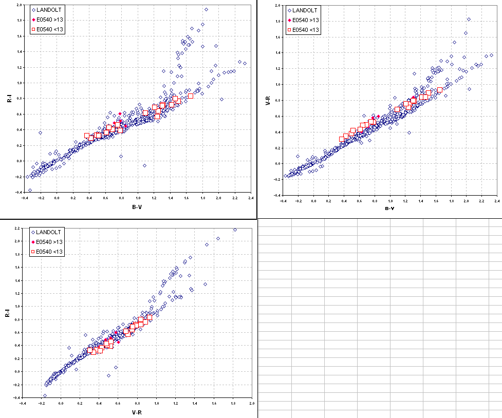
Figure 3. Star colors scatter diagram for 707 Landolt stars and the 24 E0540 stars that were "solved" using my equation algorithm.

This graph is a "sanity check" meant to uncover systematic errors in the solutions for any of the 4 magnitude bands for the unknown region E0540. The E0540 stars exhibit small offsets with respect to the Landolt stars. This could be caused by changes in extinction between the time the Landolt area was observed and the time E0540 was observed. It could also be caused by an error in my assumed extinction combined with the fact that the E0540 ROI was observed when it was at a slightly different air mass than the Landolt area. A third possibility is that my filter wheel doesn't stop at the same location each time a filter is selected, and the slight mis-alignment causes a slightly different flat frame (indeed, I found evidence for this when exposing the flat frames: the appearance of the flat frame image depended on the direction from which I approached a specific filter). Whatever the explanation, it is appropriate to make use of the extra information about star colors to apply empirical adjustments to the equation magnitudes in order to achieve agreement with the Landolt color/color scatter diagrams. When this is done we obtian the following color/color scatter diagrams.

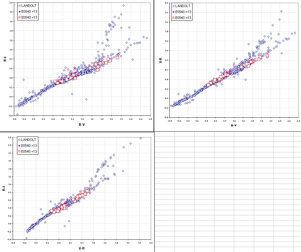
Figure 4. Star colors scatter diagram for 707 Landolt stars and the 24 E0540 stars that were "solved" using my equation algorithm. Adjustments of +0.04, -0.03, 0.00 and 0.00 were applied to the E0540 BVRI magnitudes.

These color/color scatter diagrams were obtained by applying empirical offset corrections to the B- and V-band magnitudes for E0540. The corrections are +0.04 and -0.03 magnitude. No corrections for the R- and I-band magnitudes were necessary.

2004 Dec 01 All-Sky Observations

On December 01, 2004, UT, I used a Celestron CGE-1400 (14-inch Scchmidt-Cassegrain) telescope in a prime focus configuration using a Starizona HyperStar field-flattening lens. I used a SBIG CFW-8 with Custom Scientific BVRI filters attached to a SBIG ST-8XE CCD camera. During the course of 9.3 hours I observed 3 Landolt regions and two exoplanet regions for the purpose of creating a BVRI photometric sequence for the exoplanet star fileds.

The Landolt regions were LA2343 (16 stars, m ~ 1.2), LA0452 (31 stars, m ~ 4.1, 3.1, 2.4, 2.1, 1.6), LA 9853 (27 stars, m ~ 1.8), where LA2343 refers to the Landolt star group at RA = 23:43 (Dec ~ 0) and "m" is a synbol I've used for decades in the atmospheric sciences to represent air mass. For the B-filter there are 198 observations (of 74 Landolt stars), for the V-filter there are 105 observations (of 74 stars), and for the R- and I-filters there are 30 observations (of 23 stars). All "intensities" were hand measured (locating the aperture pattern for maximum intensity for the bright stars, and centered viisually for the faint stars) using MaxIm DL 4.0.

Measured intensity was converted to magnitude using the following equations:

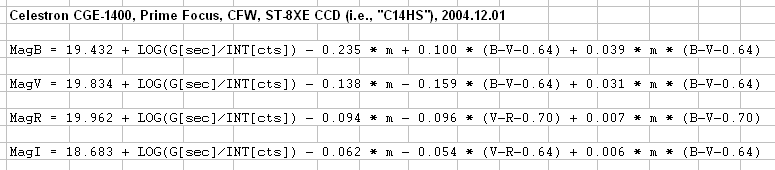
 Figure 1. Equations used to convert measured intensity to magnitude. G is exposure time [seconds], INT is measured intensity (using photometry aperture settings of 6, 2 and 7 pixels (radius for signal aperture, gap width, sky background annulus width), m is air mass (from TheSky 6.0), B-V are from the Landolt listing, and all coefficients were determined using a least squares procedure.

In the above equations the first coefficient has to be adjusted from one night to the next for reasons that I don't fully understand (for example, they can be influenced by dust on the aperture corrector plate). The second coefficient is extinction [magnitudes per air mass], and it also must be adjusted from one night to the next (provided there is sufficient air mass coverage to warrant an extinction solution). Note that extinction declines with wavelength, as it should. The next coefficient is related to star color, and it should be the same for a given telescope configuration. Whenever the Landolt stars exhibit a large range of star colors I adjust this coefficient. The alst coefficient is related to the fact that star color varies slightly with air mass.

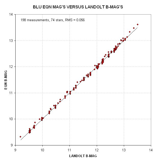
Figure 2. Equation B-magnitude from 198 measured intensities of  74 Landolt stars versus Landolt B-magnitudes. RMS scatter is 0.056 magnitude, which assumes extinction was constant throughout the observing session.

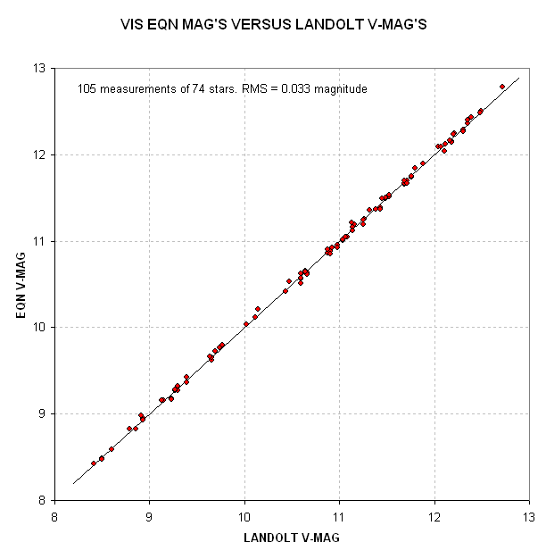
 Figure 3. Equation V-magnitude from 105 measured intensities of  74 Landolt stars versus Landolt V-magnitudes. RMS scatter is 0.033 magnitude (which assumes extinction was constant throughout the observing session).

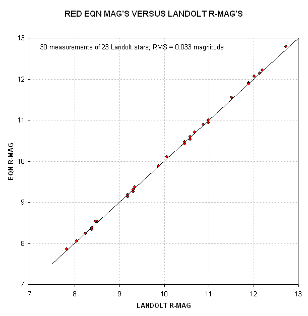
 Figure 4. Equation R-magnitude from 30 measured intensities of  23 Landolt stars versus Landolt R-magnitudes. RMS scatter is 0.033 magnitude (which assumes extinction was constant throughout the observing session).

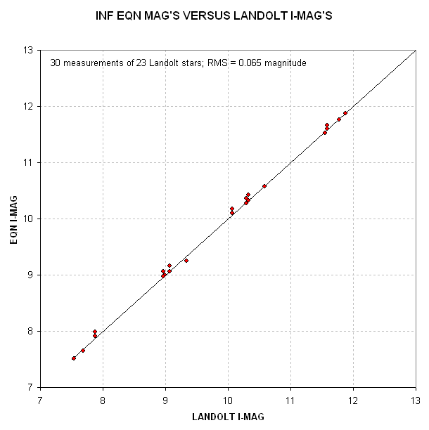
 Figure 5. Equation I-magnitude from 30 measured intensities of 23 Landolt stars versus Landolt I-magnitudes. RMS scatter is 0.033 magnitude (which assumes extinction was constant throughout the observing session).

The extinction solution for the 9.3-hour observing session is shown in the next graph.

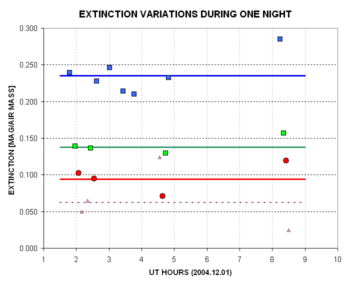
 Figure 6. Extinction versus time for B, V, R and I-bands. The average values are 0.235, 0.138, 0.094 and 0.062 magnitude per air mass.

The extinction plots for B, V and R are correlated, going down then up. They appear to undergo a similar percentage variation, as the next graph shows.

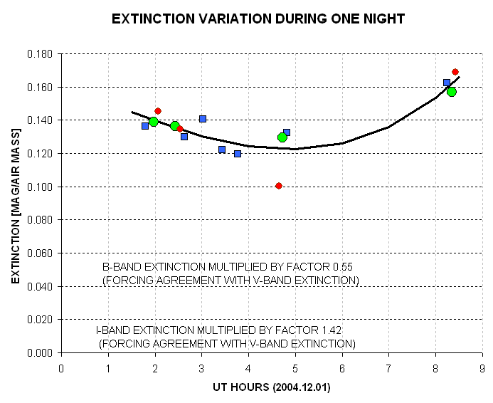
Figure 7. Extinction versus time for B, V and R-bands for which B-band and R-band extinctions were multiplied by factors that made them approximately equal to the V-band extinction. The same curved shape appears for all 3 bands, consistent with the idea that extinction underwent a variation that had the same percentage amplitude at all wavelengths.

The amount of variation of apparent extinction in the above figure is difficult to explain. A cirrus cloud would produce the same increment of absolute value for extinction at all bands, not a similar percentage change. The B-band shows a greater increase than the other bands. I simply don't understand the systematic changes, so I adopted average values for the analysis at the risk of increasing scatter in the equation magnitudes for not properly representing extinction variations. This may account for the uncommonly large RMS scatter in Fig.'s 2 and 5 (B-band and I-band).

When the set of 24 unknown stars in the E0540 field are plotted in a B-V versus V-R scatter diagram it is possible to detect when an offset error is present in the equation magnitude solutions. The same can be said for a scatter plot of V-R versus R-I. By comparing the equation magnitude scatter patterns with the corresponding scatter pattern for the 1200 Landolt stars it is possible to perform a "reality check" that can reveal the need for additional empirical magnitude offset corrections to the unknown stars. When this was done for the 47 E0540 stars it was found that adjustments of +0.190, -0.110, +0.020 and -0.015 magnitude were needed to shift their scatter pattern so that they overlapped the landolt pattern. This set of adjustments is close to a minimum adjustment set, and it is uncomfortably large. The large shifts show that something went awry in the all-sky calibration process. I suspect that my handling of extinction may be the flaw that produced the need for such large shifts. The final magnitudes that I adopted have colors shown in the following two graphs. 

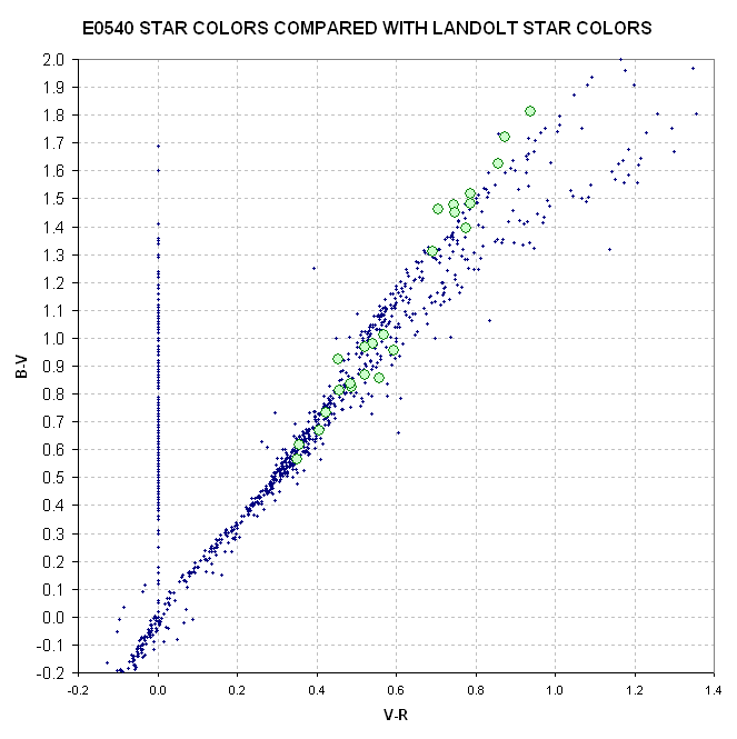
Figure 7. Final solution for E0540 star colors (B-V versus V-R) compared with Landolt star colors, after applying empirical adjustments.

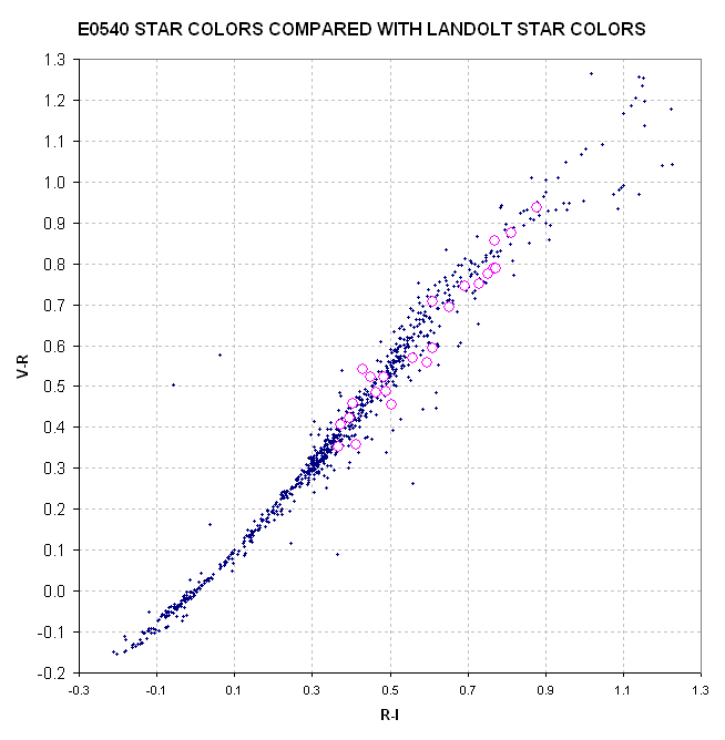
Figure 8. Final solution for E0540 star colors (V-R versus R-I) compared with Landolt star colors, after applying empirical adjustments.

After considering the size of the empirical shifts applied to B, V, R and I mequation magnitudes, and also considering the RMS scatter in the equation magnitude versus Landolt magnitude plots, I have adopted the following SE uncertainties for the 47 E0540 stars:

Re-Analysis Deducing Source of Mysterious Extinction Variation

After completing the analysis described above, I investigated the mysterious anomalies that caused variations in apparent extinction. I paid special attention to the possibilities of "hoarfrost" on the following optical surfaces: 1) telescope front corrector plate, 2) filters, 3) CCD cover plate and 4) CCD chip. Each hoarfrost hypothesis could be rejected based on expected "behaviors" and I finally concluded that the culprit was a thin cirrus haze that covered the sky and grew slowly during the night. It will be useful to explain how I arrived at this conclusion, as it illustrates the importance of a simple precaution that I shall adopt for all future all-sky observations.

In the past I've been fooled by the slow accumulation of dew on the telescope front corrector plate. It usually happens after a rainy day, when the air is humid from ground water evaporation. Frost formation follows the same setting; the only difference being ambient temperature (frost point is essentially the same as dewpoint for surface pressures). I monitor dew point and ambient air temperatrue, as well as telescope tube temperature (to support my use of a focuser), and on the night in question the two temperatures differed by ~16 F. This renders it very unlikely that hoarfrost formed on the telescope front corrector plate. Additional evidence for ruling out this hypothesis comes from the fact that the anomalous extra extinction exhibited a dependence on elevation angle (air mass), as described below.

On this night I set the CCD cooler to -30 C, which is the coldest I have ever used. In the past I have noted a "fog" come over images when I set the CCD TEC cooler to cold and the last time I baked the CCD dessicant unit was last summer, during the monsoon season. I recall feeling brave when I set the coolr to -30 C. If either the CCD cover plate or the telescope corrector plate had acquired a thin coating of hoarfrost it would have reduced the amount of light reaching the CCD chip and this might have mimicked a change in atmospheric extinction. If frost did accumulate on the CCD chip, or cover plate, or filter, the decreased transparency of the surface would be associated with an increased sky background level. The following graph shows the sky background level measured for non-star regions of 14 B-filter images.

This graph seems to support the idea of frost accumulation, until 06 UT, followed by a slower evaporation. The shape of this trace is somewhat consistent with the outside air temperature, which reached a minimum of 20 F at 06:20 UT and began to rise at 08:00 UT. The telescope aperture can be colder than the ambient air since it can radiate IR photons to cold space more efficiently than the layer of air close to the ground (since the thermal IR emissivity of the telescope tube is much closedr to one than the layer of air). However, a sensor on the telescope tube (close to the rear, where the focuser motor is located) registered 21 F (-6 C) at about 7:45 UT. To speculate that hoarfrost formed on the telescope front corrector plate would require that my dew point sensor was inaccurate by ~15 degrees. this is unlikely based on other times (albeit warmer) when foggy surface conditions were associated with dew points close to ambient temperature. 

If frost accumulates on the CCD cover plate, or the chip itself, it will start with condensation sites which grow with time. Never, in my experience, has a too-cold chip produced a uniform pattern of "fogginess." Invariably a mottled pattern appears, and grows noticeably with time. There was no evidence of this, so I doubt that frost formed on either the CCD chip or nearby cover plate. If, instead of frost forming on the chip or cover plate, frost formed on a filter (which is a few millimeters from the cover plate) the mottled pattern of condensation sites would not be as noticeable. More time was spent observing with a B-filter than the others, as I wanted to do a good job of establishing B-band extinction for my site and this observing session afforded a good opportunity with a couple hoursof free time before the exoplanet fields could be observed. If the B-filter was more frosted than the other filters, then I should see a different amount of sky background enhancement for images taken with the other filters, and their pattern of enhanced background versus time could be different. To pursue this line of thought I measured sky background for the R-filter images, thinking that it should be much less and more constant considering the better RMS scatter of Equation R-magnitudes versus Landolt R-magnitudes scatter diagram (Fig. 4, above).

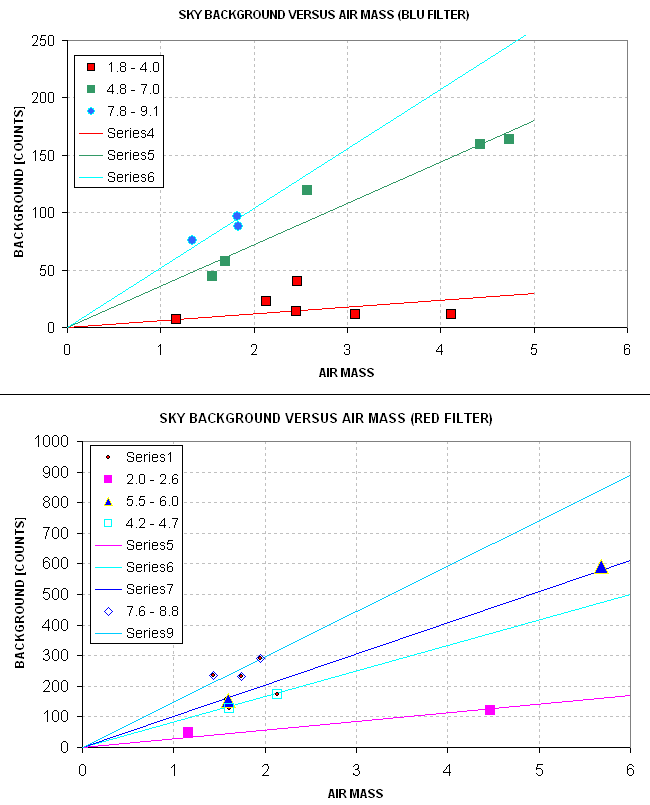
Figure 10. Background sky levels for non-star regions near the center of images taken with a B-filter (top panel) and R-filter (bottom panel). Data taken close to each other in time are assigned different colors, and a hand-fitted slope is shown that corresponds to a linear dependence with air mass.

I was surprised to learn that the R-band images had larger sky level enhancements than the B-band images. Furthermore, when the background levels are grouped by time intervals, they exhibited a lienar dependence upon air mass. This behavior is consistent with the presence of cirrus clouds that covered the sky. The following graph is a plot of the slopes of the lines in this graph versus time.

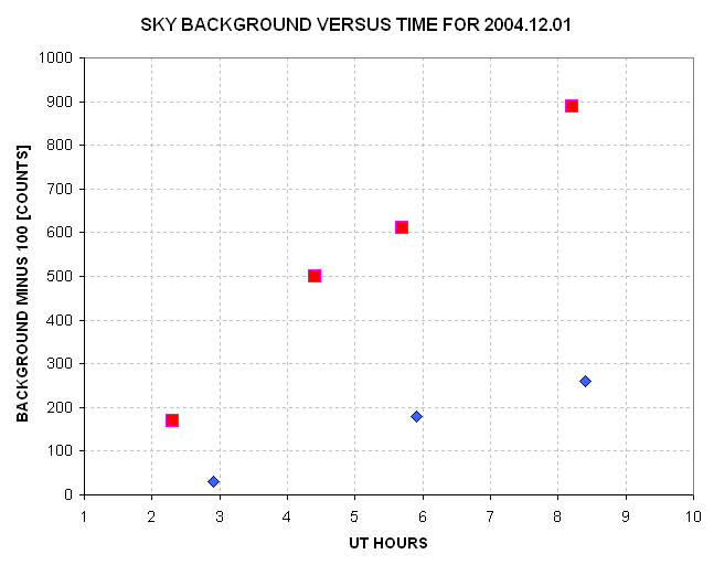
Figure 11. Slopes of "sky background level versus air mass" plotted versus time. The R-band slopes (red squares) are aboput 3.6 times greater than the B-band slopes (blue diamonds).

I was unable to obtain satellite IR images for this date since they are not archived for public doain access. The radiosone profile from nearby Tucson at 12 UT showed a 6 C dew point to ambient difference just below the tropopause (where cirrus clouds usually form), and the Yuma sounding showed a trend toward that condition before its dew point sensor failed. Radiosonde dew point measurements are notoriously inaccurate at high altitudes, so we merely have semi-confirmation that cirrus clouds were present in Southern Arizona during this night. At sunrise the next day (14 UT) I didn't notice cirrus. Figure 7 implies that extinction was NOT increasing monotonically during the night.

I take the position that I DO NOT KNOW what caused the unusual behavior for both the extinction measurements and the sky background level measurements. Although I favor the cirrus hypothesis, I really don't need to know, since neither explanation will allow me to "rescue" the observations from this night for credible all-sky photometry results. I plan on another attempt at all-sky observing for creating a photometric sequence for thses two exoplanet star fields.

Whether the enhanced sky background levels in the images were due to cirrus or due to hoarfrost, the observations should be thought of as "non-photometric." It is important to monitor photometric conditions when attempting to conduct photometric observations. The principal "take-home lesson" from thhis long and arduous analysis can be summarized by the following:

    MONITOR SKY BACKGROUND LEVELS WHEN CONDUCTING ALL-SKY OBSERVATIONS

Link to Concepts for All-Sky Photometry (describing the reasoning underlying the procedure for deriving Equation Magnitudes)

This site opened:  December 6, 2004.  Last Update:  December 23, 2004