Mosaic Flat Fields
Bruce Gary,
Last updated 2013.06.28
The following experiment was motivated by
the need to understand why a set of moving asteroid images
weren't producing good results. I quickly identified the
problem to be related to a bad master flat field. The master
flat was made in the usual way, using a T-shirt diffuser at
dusk. However, it was found to include a large component of
reflected light, based on tests of internal consistency, to
be explained in this web page. Even worse, the master flat
that I determined by imaging the same star at 54 locations
in the FOV showed that the real flat field should correct
for stars being brighter near the edges of the FOV, not the
center - as would occur if vignetting were important. This
web page is therefore a "lessons learned" story of my
floundering to figure out a good way to correct the effects
of a bad master flat field.
Introduction
A flat field correction is needed to reduce the effects of 1)
responsiveness of individual CCD pixels to photon flux, 2) dust
donut shadows and 3) vignetting (and related effects) affecting
star flux across the CCD. For making "pretty pictures" it is
acceptable for the master flat to include the effects of
reflections (i.e., from a nearby moon, bright star, street light,
etc). For differential photometry of a star undergoing brightness
changes, such as undergoing the transit of an exoplanet, the
master flat's reflected light component won't matter, provided the
star field is fixed with respect to the pixel field (by using an
autoguider, for example). However, for a moving asteroid the
reflected light component should be removed from the master flat -
somehow. This is because reflected light doesn't affect the
transmission of a star's light through the telescope optics.
This web page was prompted by the significant difference between
a flat field produced in the standard way and a flat field that
leads to uniform star response across the FOV, as illustrated by
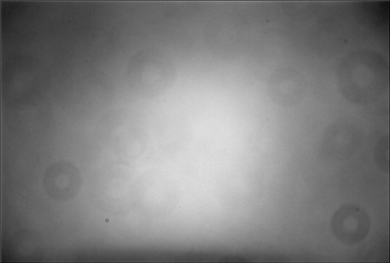
the following pair of flat fields:
 vs.
vs. 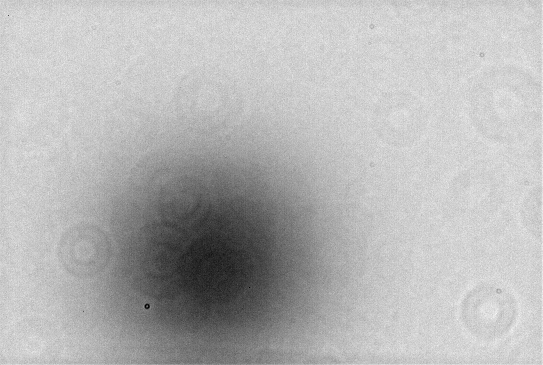
Figure 0.1. Left panel: Flat field produced in the
traditional way (diffuser over aperture during dusk). Right panel:
Flat field produced by a complicated procedure that assures
uniform response to star brightness across the FOV.
Images calibrated using the standard flat field look good, and this
is what should be done for pretty picture tasks. But these pretty
images have the drawback that a star placed at a 9x6 matrix of
locations exhibits a 220 mmag variation in brightness. When the flat
field in the right panel of the above figure is used the range of
brightness values is greatly reduced. Using an even better approach
(neglecting to include a flat field in the calibration and solving
for correction equations to provide uniform response) reduces the
range of variation across the FOV such that residuals exhibit a SE
uncertainty of ~ 8 mmag.
The path to my recommended procedure is complicated, but the dead
ends are instructive. I've chosen to describe the various attempts
to solve the flat field problem in the form of chapters.
Chapter 1: Naive Use of Dusk Master Flat
This story begins with the failure of my 14-inch Meade LX-200 a
week before planned observations of asteroid 285263 (1998 QE2). I
had shown with my Meade that the Optec focal reducer was
significantly superior to the Meade brand focal reducer in terms
of having a much lower light reflection component in master flats.
This is shown in the next figure for 6 filters.
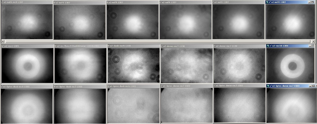
Figure 1.1. Top row is a set of master flat fields with
no focal reducer for use of filters, u', B, V, g', r' and z'.
Middle row is for use of a Meade brand focal reducer. Bottom row
is for an Optec focal reducer, that has several layers of
coatings to reduce reflections over a large range of
wavelengths.
If you're going to use a focal reducer it's worth the cost of
buying a good one.
With my Meade unrepairable in time for the asteroid observations
I was forced to use a 11-inch Celestron CPC-1100, my "backup
telescope." I didn't have an Optec focal reducer (FR) for it, so I
used the Celestron FR. The incentive for using a FR with a moving
asteroid is to minimize the number of FOV moves during an
observing session.
The Celestron flat field, produced with a T-shirt diffuser at
dusk, is shown below.
Figure 1.2. Dusk master flat field, without FR, using
T-shirt diffuser at dusk.
This flat field looks like every other one I've taken in overall
structure; the corners are darkest suggesting that stars should
appear fainter there due to vignetting. The master flat for a
configuration including the focal reducer was qualitatively the
same, but more extreme (even darker in the corners). This is to be
expected since vignetting should be worse with a focal reducer.
After a few nights of observing the asteroid I was obtaining
image sets for several FOV placements. It bothered me that the
light curve (LC) segment for each FOV placement looked the same: a
deep U-shaped LC. So I removed the FR and found that the U-shapes
flattened out - but not entirely!
This called for an evaluation of systematics versus location
within my FOV, and the only way I could think to achieve that was
to observe an open cluster of calibrated stars and empirically
determine what a master flat pattern should be.
Chapter 2: Open Star Cluster Calibration
I chose NGC 5466 because it "filled" my FOV with stars that were
calibrated for my r' filter band. It had both CMC14 and APASS
magnitudes at r'-band, but I had shown elsewhere that the APASS
r'-band magnitudes were superior (smaller scatter with my fits).
Here's an example of a model fit to "Obsd mag minus True mag vs.
Star Color".
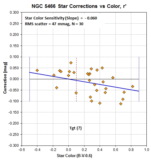
Figure 2.1. Comparing observed with catalog r'-band
magnitudes fitted by a linear model. Most of the scatter
is due to the use of a standard flat field that is flawed due to
the presence of reflected light.
The differences with respect to the model fit, above, are plotted
versus distance from the center of the FOV (actually a location
slightly displaced from the center, to a location that is the peak
of the master flat function), as shown in the next graph.
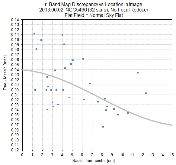
Figure 2.2. Differences (from previous figure) plotted
versus distance from FOV "center."
A pattern in these differences is apparent, with stars near the
center being too faint. This pattern ranges from ~ -40 mmag at the
center to ~ +60 mmag near the edge. In other words, unless
something is done to correct the problem the asteroid will appear
to fade ~ 100 mmag while approaching the FOV center and then
regain ~ 100 mmag in brightness as it moves to the opposite edge.
This is unacceptable!
As a temporary solution I adjusted the master flat in clever ways
to remove this 100 mmag pattern, and proceeded to show that new
versions of the above figure were "flat." The scatter on the
empirically adjusted star magnitudes was ~ 15 to 20 mmag, so that
at least was acceptable for determining the asteroid's 200 mmag LC
variation.
Chapter 3: Mosaic Master Flat
MaxIm DL has a "mosaic sequence" option meant for pretty picture
people. I used it to create a set of images that placed the same
star at locations 2' arc apart in RA and DE, using a 9 x 6 raster
pattern. These 54 star locations nicely sample my entire FOV. I
chose a star that was near zenith to minimize atmospheric
extinction changes during the 25-minute mosaic sequence. It's
magnitude allowed for 6 second exposures. Brighter stars would
require shorter exposures which would have increased scintillation
noise. No flat frame calibration was performed; only dark frames
were used. Here's an average of the 54 image set.
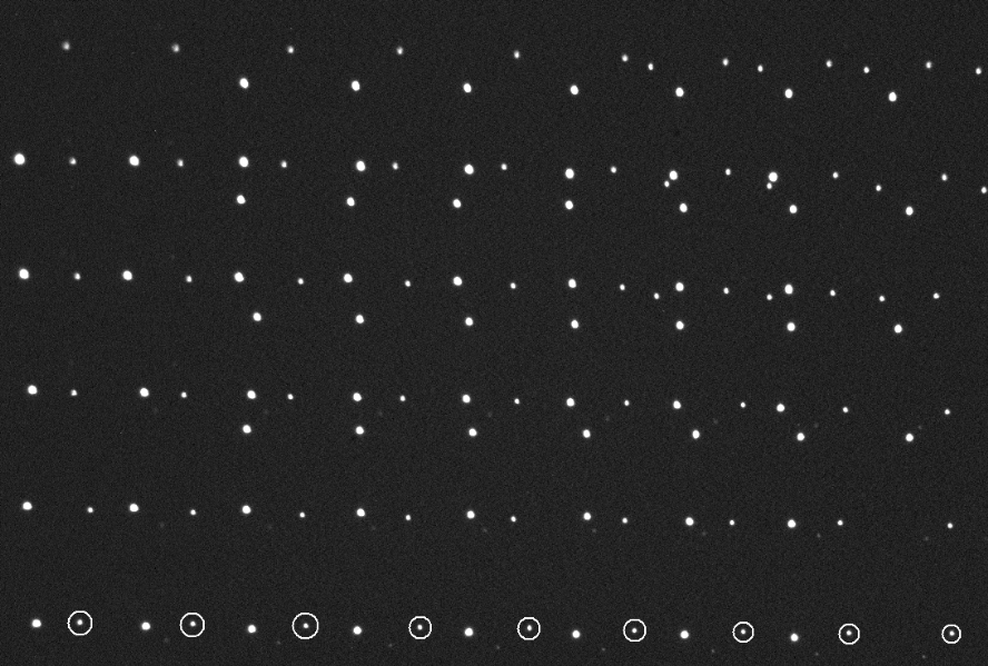
Figure 3.1. Pattern of locations within FOV of star
chosen for analysis (bottom row locations, circled). Other stars
are present but were not used. MaxIm DL performs a 9x6 set
of observations in 25 minutes (6 seconds exposure time). This
is an average of the 54 image set.
Manual readings of x/y location and magnitude were entered into a
spreadsheet (top panel of next figure).
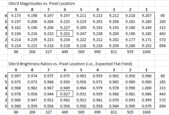
Figure 3.2. Top panel: Pattern of
magnitudes of star chosen for analysis versus FOV pixel location.
Pixel locations are given at bottom row and right column. Bottom
panel: Same data converted to brightness relative to the brightest
value (which is in the upper-left corner). The cell where the star
appeared faintest is indicated (near the middle). These data are
for a configuration without the focal reducer and a calibration
that does not include use of a master flat.
The brightness pattern in this figure is surprising! It is not
unexpected, based on Fig. 2.2, showing that "apparent minus true"
magnitude is greatest near the center (i.e., stars appear fainter
near the center). However, these data were obtained with a
configuration that produced an observed master flat field that was
darkest in the corners (c.f., Fig 1.2), where vignetting should
cause stars to appear fainter. How can stars appear brightest near
the corners?
Let's forge ahead as if all discrepancies can be accounted for by
invoking a large component of scattered light in the observed master
flat, causing it to appear brightest near the center even though
that's where stars appear faintest.
Another way to present the same data in the previous figure is to
show differences from the brightest magnitude (top panel of next
figure).
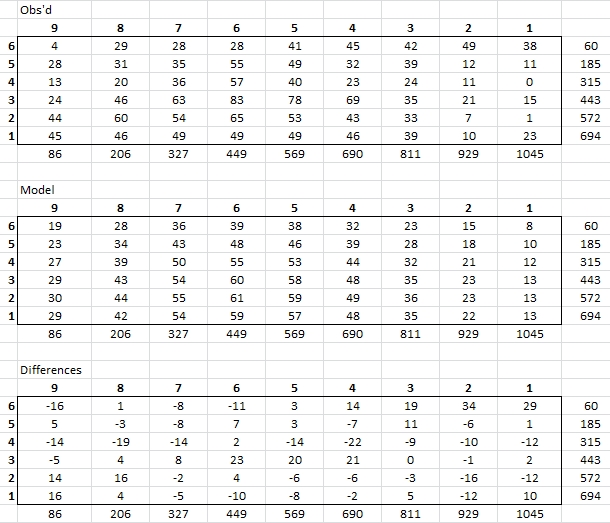
Figure 3.3. Table of same star FOV magnitude
differences [mmag] without use of a FR and without using a flat
field during calibration (only dark). Top panel shows values
of "apparent magnitude minus the brightest value" of one star at a
9x6 matrix of locations in the FOV. The middle panel is a model
fit to the top panel, consisting of a Gaussian shape, described in
the text. The bottom panel shows "observed minus model"
differences. All values are in mmag units.
The 2-dimensional (2-D) Gaussian function is centered at x/y =
475/558 (which is near the middle of a 1092x736 FOV). The 1/e widths
for x- and y-directions are 548 and 749 pixels. A multiplier of 61
mmag provided the Gaussian magnitude scale.
The RMS scatter of the bottom panel is 12 mmag, suggesting that the
use of a 2-dimensional Gaussian for flat field correction should be
possible with this accuracy. The RMS scatter of "same image location
measurements" is ~ 5 mmag, so the 2-D Gaussian representation is
missing some real structure. Additional terms might have to be
included eventually.
Notice that the top panel shows that the star was fainter near
the middle of the FOV than near the edges. This agrees with the
previous analysis, using APASS magnitudes for NGC 5466. The total
range of the top panel is ~ 80 mmag; the range for the 2-D
Gaussian is ~ 50 mmag. The 2-D Gaussian model isn't perfect, but
it "points the way" to a more sophisticated model when the quality
of mosaic calibration data warrants it.
In theory this 2-D Gaussian flat field correction could be used
by applying only a dark (and bias, if needed) calibration to all
asteroid images. This could be implemented by specifying the
starting and ending x,y FOV locations in a spreadsheet for each
FOV asteroid track, and calculating for each photometry reading
the Gaussian flat field correction.
But there's a potential problem with this procedure. It does not
allow for the removal of the pattern of dust donuts or
pixel-to-pixel response differences. One could argue that these
two missing corrections would merely add noise for a fast-moving
asteroid, since so many pixels are involved in a set of images for
each FOV placement. Still, let's see if we can do this right, and
apply a standard master flat field followed by a 2-D Gaussian
(plus other terms) empirical correction based on a mosaic
sequence. That's the goal of the next chapter.
Chapter 4: Standard Master Flat Plus Mosaic Flat Correction
The set of 54 images described above were subjected to a
calibration correction using a standard master flat field obtained
at dusk. The manual measurements of the 9x6 mosaic set of images
were repeated, and here's the spreadsheet display of needed
corrections.
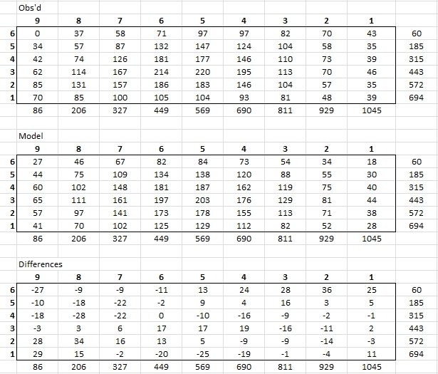
Figure 4.1. Table of same star FOV magnitude differences
after using standard master flat field during calibration. Top
panel shows values of "apparent magnitude minus an arbitrary
value" of one star at a 9x6 matrix of locations in the FOV. Pixel
location values are shown at the bottom and right sides. Middle
panel is a model fit to the top panel, consisting of a Gaussian
shape, described in the text. Bottom panel shows "observed
minus model" differences. All values are in mmag units.
The 2-dimensional (2-D) Gaussian function is centered at x/y =
530/429 (which is near the middle of a 1092x736 FOV). The 1/e
widths for x- and y-directions are 414 and 393 pixels. A
multiplier of 205 mmag provided the Gaussian magnitude scale. This
multiplier is 3.4 times greater than the one that fits the data
without use of the standard master flat. The increase was expected
because the reflected light pattern produces a central
brightening.
The RMS scatter of the bottom panel is 17 mmag, suggesting that
the use of a 2-dimensional Gaussian for flat field correction
should be possible with this accuracy. The RMS scatter of "same
image location measurements" is ~ 5 mmag, so the 2-D Gaussian
representation is missing some real structure. Additional terms
will eventually be added. The 17 mmag RMS scatter off the Gaussian
model is larger than the 5 mmag RMS scatter for the case of not
using a standard flat field during calibration.
The fact that RMS is worse when a standard master flat is used in
calibration means that the improvements associated with removing
donut effects and pixel response differences was less important
than the inability to easily fit the superposition of the
reflected light pattern and star response patterns. If the
worsening RMS scatter with respect to the 2-D Gaussian model can't
be overcome by extra terms in the model then the use of a standard
flat field during calibration should be viewed as an inferior
processing procedure than the procedure that doesn't include use
of the flat field.
Chapter 5: Two Choices for Improving Flat Field Correction
One method for correcting photometry measurements of an image set
that did not include a flat field during the calibration is to
apply correction equations to these measurements using their x,y
FOV location and the 2-D Gaussian solution described in chapter 3.
Another method is to create a master flat that incorporates the
2-D Gaussian corrections needed. This second approach is the
subject of this chapter.
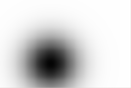
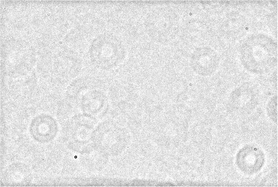
Figure 5.1. Left panel: A 2-D Gaussian that
approximates the required corrections determined in Chapter
3. Right panel: High spatial frequency structure that
should be added to the 2-D Gaussian patter in constructing a
final master flat field.
The above figure's left panel was constructed starting with an
artificial star, and enlarging it until it had the desired pixel
width. It was then multiplied down and 50,000 counts were added,
such that the ratio of fluxes at the center of the Gaussian to a
location in the white area was 0.945 (corresponding to the mmag
range determined in Chapter 3). The right panel was obtained
by smoothing the standard master flat (e.g., Fig. 0.1a, or Fig.
1.2), and then subtracting the un-smoothed image from the smoothed
one. When the two are added we get the following master flat:
Figure 5.2. A master flat that includes the 2-D Gaussian
(c.f., Ch. 3) and the high spatial frequency image (c.f., Fig
10b).
The high spatial frequency component is desirable because it
contains information about dust donuts and pixel-to-pixel response
differences.
Several steps are missing in the above description of how the final
master flat was produced, and the details aren't important; but I do
want to register that the process is fairly complicated.
When the same 9x6 mosaic image set was calibrated using all the
normal elements (bias, dark and master flat), and photometry
readings were made and entered into a spreadsheet, there was an
improvement in the uniformity of star brightness across the FOV.
However, the RMS residuals were worse than those found using the
flat field correction equations in Chapter 3 (18 mmag vs 8 mmag).
This may be due to the fact that the Gaussian had the same width in
x- and y-directions, whereas the flat field correction equations
allowed for different Gaussian widths. It would be complicated to
add this extra feature; just as it would be complicated to add any
other correction equations that could result from a refined Chapter
3 analysis (such as Fourier terms). I therefore abandoned this this
strategy.
Chapter 6: Elaboration of "Flat Field Correction Equations"
Recall that the Chapter 3 procedure included only master dark and
bias frames for image calibration. Since we now have a "high spatial
frequency image" it can be included in the calibration procedure,
which might lead to a slightly lower noise level in photometry
readings. We can't call it a flat field, however, until adding a
uniform field of ~ 50,000 counts (the approximate level for the
standard master flat). Of course, such a flat field neglects low
frequency spatial structure, such as vignetting and reflections, but
it removes some of the contributions that could interfere with our
search for the desired "low spatial frequency structure" of what
we're trying to solve for: flat field for star brightness
uniformity."
Incidentally, the "high spatial frequency flat field" will not
change if collimation is adjusted, whereas vignetting and reflection
components will change. This is a useful property to keep in mind.
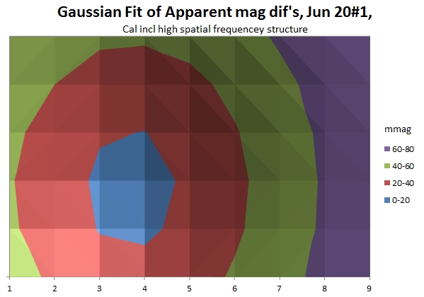
Figure 6.1. Surface plot of Gaussian 2-D fit to apparent
magnitude variation across FOV. This is a "bowl" shape,
with faintest brightnesses in the middle blue region.
Another way to present the same data in the previous figure is
shown below:
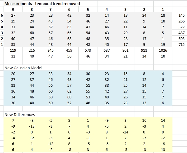
Figure 6.2. Table of same star FOV magnitude
differences [mmag] after calibrating with a master flat that
includes the high spatial frequency structure. Top panel
shows values of "apparent magnitude minus the brightest value"
of one star at a 9x6 matrix of locations in the FOV. The middle
panel is a 2-D Gaussian model fit to the top panel (same data
used in the surface plot, Fig. 6.1). The bottom panel
shows "observed minus model" differences. All
values are in mmag units.
The bottom panel of this data shows that the 2-D Gaussian model
represents the "flat field corrections" with a RMS scatter of 6.4
mmag! This is an improvement over the analysis that neglected the
high spatial frequency structure (8 mmag), so I conclude that it
is worth including the high spatial frequency structure as part of
the flat field calibration.
Chapter 7: Verifying Mosaic Flattening Equations
This chapter is actually an internal consistency check because
we're going to use the equations for flattening star brightness
response, the "mosaic-based flattening equation" to flatten the 54
measured magnitudes of a star from the 9x6 mosaic observing
sequence used to generate the MFE equation.
Here's a sample MFE:
 (eqn 1)
This equation, which I'll refer to as MFE (mosaic-based
flattening equation), uses an offset that converts magnitude
readings at any x,y FOV location to a magnitude that would have
been measured if the star had been at the center of the FOV
(546,368).
When the above equation is applied to the 9x6 mosaic's 54
measured magnitudes, a temporal variation is derived, given below:
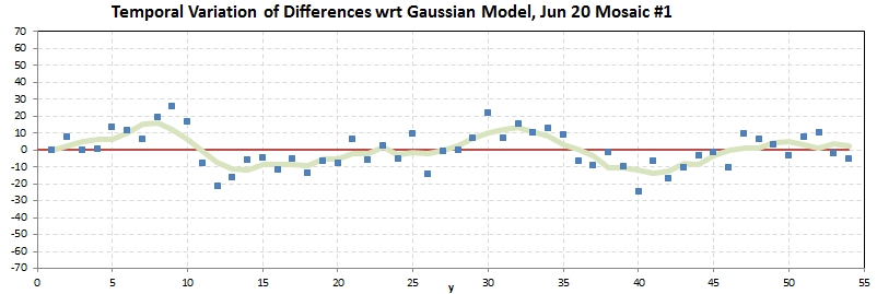
Figure 7.1. Temporal variation of a star's MFE-corrected
magnitude versus time, during the 25-minute observing sequence.
The magnitude scale is in mmag units.
After removing the above variation the following scatter plot is
obtained.
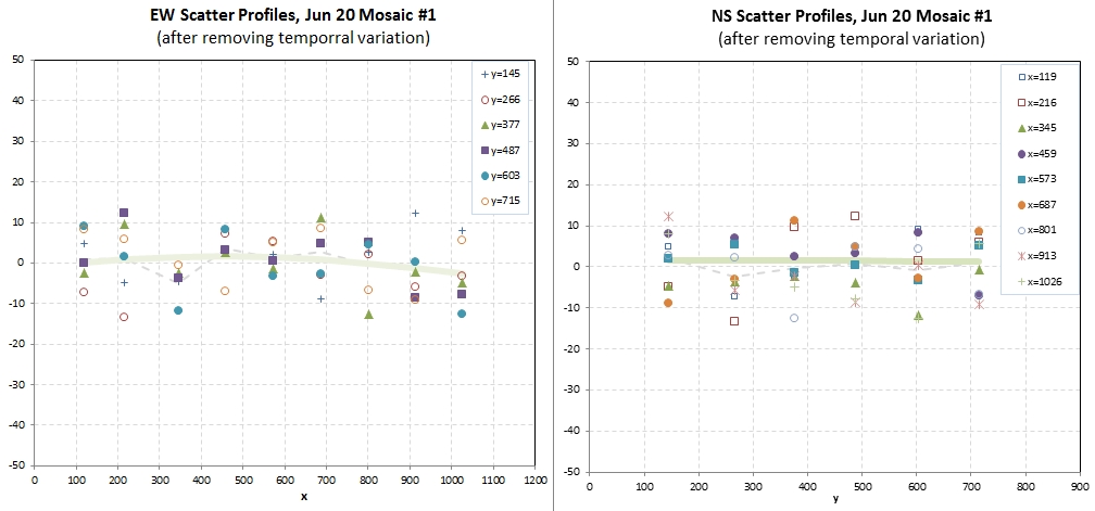
Figure 7.2. Scatter plot of differences between observed
and model predicted magnitudes for 54 images of a 9x6 mosaic.
The RMS scatter from this analysis is 7.1 mmag, so I conclude
that the above equation has been properly derived and implemented
in a spreadsheet.
Chapter 8: Applying MFE to Asteroid Observations (FOV
Calibration)
Asteroid 1998 QE2 (285263), hereafter referred to on this web
page as QE2, passed Earth at a distance of ~ 15 times the moon''s
distance on ~ 2013.05.31. I observed it on 18 nights, for a total
of ~ 71 hours. Since it had a fast sky motion each night required
several FOV placements. I will use the June 9 observing session to
evaluate the merits of MFE.
June 9 consisted of 4 FOV placements, totaling 7.3 hours. Since I
had determined the rotation period to be 4.75 hours (on May 27)
this observing session will represent more than 1.5 rotations, and
there should be similar shapes in the rotation phase plot where
overlap exists. Because we want good joining of the 4 magnitude
plot segments, corresponding to the 4 FOV placements, it is
important to calibrate each FOV data segment using well-calibrated
stars. I have chosen to use the APASS (DR7) r'-band magnitudes
(using UCAC4), partly because they give a slightly better internal
agreement compared to use of CMC14 magnitudes, but also because
the APASS magnitudes are more easily obtained than the CMC14 ones
(using C2A instead of DS9).
FOV data set "A" consists of 168 images (binned 2x2, r'-band,
10-second exposures). I have calibrated them using a master bias,
dark and the high frequency structure master flat.
Here is an image of this "A" star field, with the QE2 path shown.
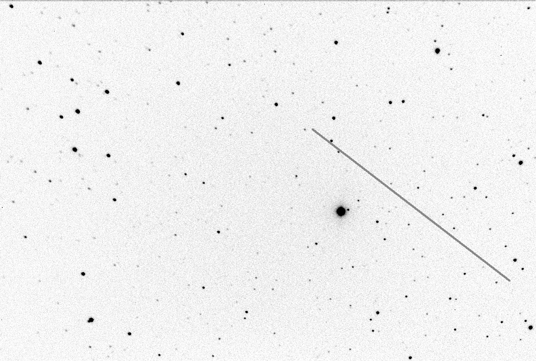
Figure 8.1. Path of QE2 during the 63-minutes of 68
images for FOV placement "A" (17:37:05 +10:03:26).
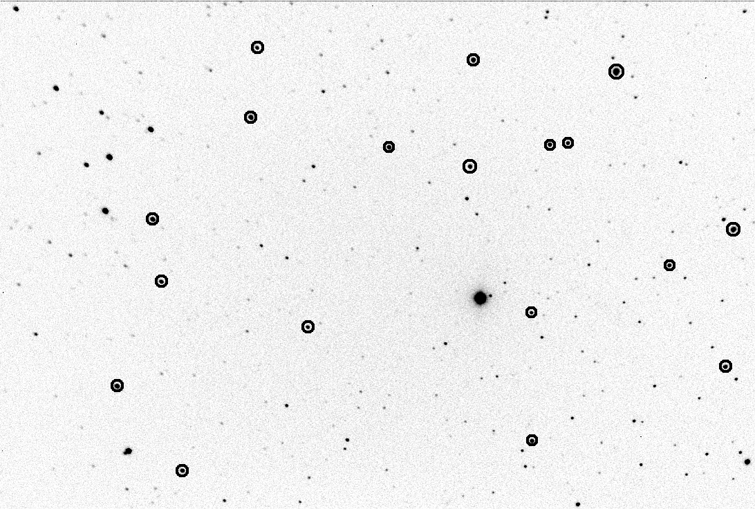
Figure 8.2. Stars chosen for setting this FOV's
"calibration" at r'-band (N=18).
x,y locations for these 18 candidate reference stars were
recorded in an observing log, for later entry in a spreadsheet. An
artificial star was placed in the upper-left corner of each image,
for use as a single "reference star." MaxIm DL's photometry tool
was used to record magnitudes for the moving asteroid as well as
the 18 candidate reference stars (assigned "check" status). You'll
notice that the collimation is imperfect, with "comet-shaped" PSFs
in the upper-left area of the FOV, and sharp PSFs in the
lower-right. The FWHM readings for the 68 images range from
~ 4.0 (3.7,4.3) to ~ 3.5 (3.3,4.1) pixels (where the 1st number is
median and the two numbers in parentheses are quartiles). Choosing
a photometry aperture has to be done carefully; if it's small
(e.g., ~ 4 pixels) it will produce a maximum SNR for faint stars
and the asteroid, but star magnitudes will be greater than actual
where PSFs are large (upper-left region of FOV). I first want to
determine whether or not my MFE produces a good calibration of the
image set. For this purpose we need to use a large photometry
aperture, such as a radius twice the median FWHM (e.g., 8 pixels).
This photometry size will produce a noisy asteroid light curve,
but it will at least be close to the correct magnitude versus
time. Smaller apertures can be evaluated for a balance of
remaining true to the overall LC plot while improving the noise
level.
A photometry radius of 10 pixels was chosen to serve as an
overall magnitude reference.
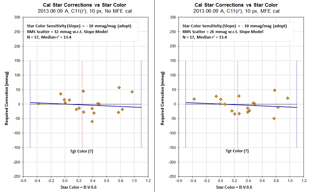
Figure 8.3. Scatter plots of APASS magnitude minus
observed magnitude versus star color showing improvement when the
MFE corrections are applied to the measured magnitude of APASS
stars.
This figure shows an improvement by incorporating the MFE
corrections for measured magnitudes, with RMS scatter going from
32 mmag without MFE to 26 mmag with MFE. I don't know what the
actual uncertainties are for r'-band APASS magnitudes, but if they
are 27 mmag for CMC14 (for r'-mag = 13.4), and if I see slightly
better internal consistency using APASS versus CMC14 magnitudes,
then the above result is a reasonable expectation assuming the MFE
calibrations were much lower (e.g., 7 mmag).
If the APASS r'-mag errors are stochastic, then the uncertainty
on the "A" FOV's calibration would be ~ 7 mmag.
Chapter 8: Applying MFE to Asteroid Observations
(Asteroid Calibration for a FOV)
The same MFE calibration can be applied to the asteroid since we
know its x,y for the first and last image in the "A" data set, and
can perform a linear interpolation for all intermediate images.
This procedure was performed for all 4 FOV segments. Here's the
combined light curve:
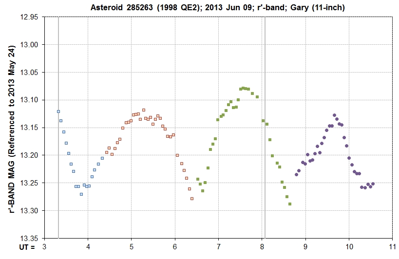
Figure 8.4. Combining the 4 FOV segments, each with an
independent r'-magnitude calibration, produces this LC spanning
1.5 rotations.
The overall pattern of two maxima and two minima is present, but
the last FOV segment looks different. What could explain this?
Consider the phase-fold LC.
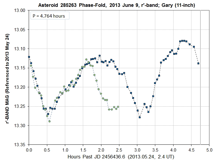
Figure 8.5. Phase-fold LC for the June 9 data, showing an
apparent "mutual event" (transit or occltation of the secondary
asteroid).
The agreement is amazingly good up to the 1.6 hour time, and
then the brightness rapidly fades, then begins to recover at ~ 2.2
hours, which the kind of behavior that would be produced by either a
transit of the secondary asteroid in front of the main asteroid, or
an occultation of the secondary by the primary.
Conclusion
The MFE procedure (mosaic-based
flattening equation) appears to work!
____________________________________________________________________
WebMaster: B. Gary. Nothing on this web page is copyrighted. This
site opened: June 18, 2013.