Introduction
Since this is the first flight that I am subjecting to analysis for this web site, it will necessarily be longer than the web pages describing analysees for the other flights. I will explain terminology, procedures, and underlying concepts in a way that will not be reproduced on the other web pages. This flight is ideal for this purpose, as it has data that produces false alarms, warning hits, and it has an altitude "dip" at the center of the flight, right in the middle of a large synoptic scale size field of CAT. This altitude dip allows a straight-forward analysis to be made of the concepts underlying my suggested approach for warning of CAT during level flight.
Overview of Flight ER911102
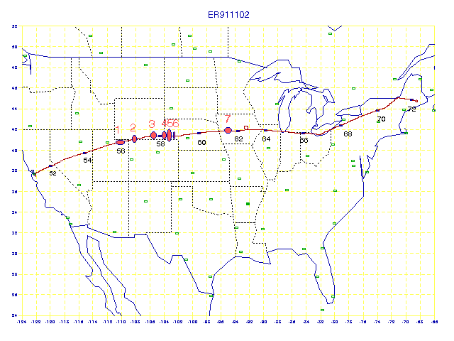
The flight of November 2, 1991 produced what the pilot reported as "Rough air from Utah to New York, light, sometimes moderate." The following is a flight track for the flight, beginning at Moffett Field, at Ames Research Center, CA and ending at Bangor, Maine.
Figure 1. Flight track for ER911102. The red ovals are CAT events, the strongest being #5. Events 3 through 6 are in an altitude dip.
The flight is especially useful for CAT studies because it includes an "altitude dip" just east of the Rocky Mountains, where CAT encounters 3 through 6 occur.

Figure 2. Flight altitude (green) and turbulence intensity, Akk (red), for flight ER911102. CAT encounters are numbered.
From this figure it is apparent that smooth flight can have Akk values less than 0.04 (i.e., <0.08 real g-units). (Akk is defined below; briefly, it's a peak-to-peak excursion of the vertical accelerometer installed in the MTP instrument, which, due to it's slow sampling rate of 1 Hz, must be multiplied by approximately 2.0 to arrive at what a high sampling rate sensor would measure.) Isolated spikes are due to such things as turns (66.6 ks) or pitch changes (e.g., 58.4 ks, better seen in a later figure, and 70.2 ks). The lower envelope of an Akk plot can also be useful in determining the reality of a CAT encounter. For example, at 61.5 ks many cycles exhibit Akk values that are always greater than 0.05, indicating that steady turbulence gradually built in intensity.
Isentrope Altitude Cross-Sections
I'll present the isentrope altitude cross-sections, IACs, in three figures (since there's so much structure to be noted in them).

Figure 3. IAC for the first third of the flight. Isentropes are 5 K apart, with the middle red trace being 480 K. Aircraft altitude is shown with a thin black trace.
Notice that isentropes begin to have structure starting at about 53.5 ks, which is over central Nevada. The dip begins at 57.5 ks, over southern Wyoming. This interval, from Nevada to Wyoming, is a region of moutain waves, having amplitudes as high as 700 meters near flight level (at about 56 ks).

Figure 4. IAC for the second third of the flight, from the Wyoming/Nebraska border to Illinois.
The mountain waves persist until about 61.2 ks, over eastern Nebraska.

Figure 5. IAC for the last third of the flight.
Some lower-amplitude waves exist over Ohio (66 ks) and up-state New York (69 ks).
Zoomed portions of some of this IAC data will be shown later in this web page.
Normal Flight "Reference"
In this web page I will first describe the dip data, as I believe it helps understand the level flight data.
Before viewing graphs of the ER911102 CAT events during the dip, it would be useful to become familiar with similarly formatted graphs of a normal flight. The earlier flight ER911004, a transit flight from California to Alaska, was reported to have only light CAT at one location. First, let's view a simple plot of aircraft altitude and "vertical accelerometer activity" versus time for a period including the altitude dip, which is normally programmed to occur in the middle of the flight. By "vertical accelermoeter activity" I mean the range of reading, taken at approximatley 1 Hz, during a data cycle (typically 10 seconds in duration). As stated elsewhere, this sampling rate is much slower than needed to capture the full intensity of turbulence, but it's what we have to work with, and I've established an empirical correction factor of approximately 2.0 to achieve agreement with pilot-reported CAT intensity. The uncorrected range of readings during a 10-second data cycle is referred to hereafter with the term Akk, for "Acceleration peak-to-peak."

Figure 6. Aircraft altitude (green) and Akk (red) verus time during a normal altitude "dip" in mid-flight.
In this figure Akk shows a 0.23 g-unit feature at the bottom of the dip, which is produced by an abrupt pitch change for terminating the descent and starting the ascent. The feature at 71.3 ks might be associated with the pitch-down transition. The feature at 73.1 ks is atmospheric-induced turbulence. The ascent is slower than the descent, which is typical.

Figure 7. Altitude profile of MTP-measured "lapse rate," defined here as dT/dZ, and Akk.
In this figure, for the same flight and for the dip only, I plot what I call lapse rate, LR = dT/dZ (opposite in sign from the conventional usage), and turbulence intensity, Akk. Dip descent data are red, and ascent data are green. The Akk data have been placed on the left margin by dividing Akk by 10 and then subtracting 13. Notice the Akk feature at the bottom of the dip. The only real Akk feature appears (green) at 18.6 km. LR differs slightly between descent and ascent, but there typically is agreement of approximately 2 K/km. The greatest difference is 5 K/km in the 18 km region. The LR structure above 19 km agrees well, even though they are separated by the greateest time interval.
ER911102
Now for the ER911102 flight's dip segment.

Figure 8. Same as Fig. 2 except for the flight of ER911102.
For this flight there was more turbulence activity, with Akk reaching 0.25 g-units (approximately 0.50 actual g-units). The Akk feature at the bottom of the dip can be disregarded. Real turbulence also exists on eaither side of the main event, just after beginning the ascent (58.6 ks) and near the end of ascent (at 59.2 ks). It is interesting that there is much more turbulence during the ascent than during the descent.

Figure 9. Same as Fig. 2, except for ER911102.
The most notable difference between this figure and its counterpart for the earlier (normal) flight is the disparity of the lapse rates between descent and ascent. During descent, where little turbulence was encountered, the LR trace (red) shows three "inversions" - with LR reaching values as high as +6 [K/km}. Later, during the ascent these same three locations are now nearly adiabatic! What could cause such a dramatic change in lapse rate? CAT!
According to my compression hypothesis for CAT generation (see Compression Hypothesis for CAT Generation) turbulence is preceded by a vertical compression, causing an inversion layer to form but also raising the magnitude of vertical wind shear, VWS, leading to a reduction oif Richardson Number, Ri, and eventually CAT. The scenario then calls for the conversion of an "inverted" temperature field to an "adiabatic" temperature field where CAT occurred and thoroughly mixed the air. CAT should uniformly mix all tracers, and since potential temperature, theta, is a conserved tracer duringt the CAT process the CAT layer should have uniform theta - which means an adiabatic temperature structure.
The descent data (red line trace) may be after the compression has begun but "before" CAT was triggered, while the ascent data (green dotted trace) may be "after" the CAT was triggered. Is this suggestion consistent with the Akk data? Yes! The most severe CAT occurred at 17.2 km, exactly where dT/dZ went from +5 or 6 [K/km] to -8 or -9 [K/km].
The smaller CAT feature at about 16 km also exhibits a switch from inversion to sub-adiabatic between descent and ascent. The third feature at 18.3 km does not lend support to this scenario.
It is worth noting that the interval of time separating passage through the same altitude is different for the three LR-change layers. For example, the lowest layer, at 16 km, is samples 6.3 minutes apart; the middle layer, at 17.2 km, is sampled 15.6 minutes apart; and the highest altitude layer, at 18.3 km is smapled 24.7 minutes apart. It is more likely that the highest altitude layer actually changed altitude, due to mountain wave activity, during the two samplings than it is for the lowest layer. A 0.2 km shift could put the two LR features at the same altitude. Another consideration related to the sampling interval is that for the longest interval layer (at 18.3 km) the turbulence might have subsided before the final sampling, which would then present itself as non-turbulent yet LR changed, which is what the 18.3 km layer shows. In fact, there is some turbulence during the first sampling, during the descent, indicating that inversion layer breakdown has begun. The other two layers appear to have commenced turbulent breakdown of the inversion layer after the first sampling.
LR Corroboration
So far I have presented a self-consistent "story" to explain the dip measurements of temperature and turbulence. There are several ways to put this story to the test.
Since the ER-2 was changing altitude the in situ OAT ("outside air temperature") measurements can be used to estimate the temperature field. I hesitate in taking the position that OAT can be used to determine T(z), since the plane does have a substantial horizontal velocity, and horizontal temperature structure is therefore influencing T(t) in a way that confuses the determination of T(z).
.png)
Figure 10. Altitude (green), temperature (blue) and turbulence, Akk (red) for a portion of flight ER911102.
Temperatures before the dip can be characterized as differing from each other with a standard deviation of 0.27 * dt0.3. For example, considering a time base of 1 minute temperatures at the same altitude are likely to differ (in a SE sense) by 0.92 K; a 10-minute time base will typically produce SE differences of 1.84 K. Bearing this in mind, the following figure, showing OAT versus altitude, is presented as an estimate of T(z):
.png)
Figure 11 OAT versus altitude during only the dip portion of flight ER911102.
At 17.2 km, the temperature profile changed from an inversion layer during descent, when no turbulence was encountered, to approximately adiabatic during ascent, when "moderate" CAT was encountered! At 16.0 km, this scenario is repeated, and corresponds to another turbulent layer during ascent. The lesser level of turbulence at 18.3 to 18.5 km has a somewhat confused temperature field, with a very shallow adiabatic layer present during descent at 18.4 km, when some turbulence is experienced. The in situ OAT data therefore support the MTP associations of turbulence with layers that change frorm inverted to adiabatic.
Level Flight CAT Encounters
Level flight CAT encounters require a different analysis from the dip encounters if they are to be used to test the "compression theory for CAT generation." During level flight we cannot infer lapse rate or vertical wind shear from in situ measurements in the manner just described (for the dip data). A new method will be used, one that was developed during the course of work for the Navy, and reported in "Clear Air Turbulence Avoidance System for the HALE Aircraft" Naval Oceanographic and Atmospheric Research Laboratory Technical Note 194, November, 1991. Since this is the first flight on this web site to be analyzed using the level flight algorithm, I will describe it in more detail than for subsequent flight cases.
The following is a repeat of Fig. 1.
Repeat of Fig. 1.
The level flight encounters are #1, 2, and 7, which surround the dip data. This is a fortuitous arrangment, since whatever characteristics apply to the dip will probably also apply to encounters #1 and 2, and perhaps 7. Specifically, the entire set of encounters is most likely mountain wave induced, containing many shallow layers that are changing from inversion to adiabatic on timescales of tens of minutes. This is a situation that I claim can be used to test the "compression theory for CAT generation."
In the case of the level flight encounters the method for testing the "compression theory" is to look for regions of rising RRi (reciprocal Richardson Number) on both sides of the CAT patch. Thus, as we approach the CAT patch we shall look for lapse rate to increase and vertical wind shear to also increase. The same pattern, but in reverse, will be searched for following passage through the CAT patch.
First, let's expand the time scale of an earlier figure to see more clearly the two level flight CAT encounters.

Figure 12. Detail of Akk and aircraft altitude for the pre-dip, level flight portion that contains two CAT encounters.
CAT encounter #1 might be two encounters, but since they are separated
by only 5 minutes, which is comparable to the warning time I claim to be
able to provide (using the Richardson Number pattern algorithm), I have
chosen to call them one CAT encounter with two maxima. After applying
the approximate correction of 2.0 to the Akk data to arrive at an estimate
of peak-to-peak vertical accelerometer excursion that would be measured
by a high sampling rate measuring instrument, CAT events 1a, 1b and 2 exhibit
2*Akk = 0.32, 0.28 and 0.26 g-units. This qualifies as "light-to-moderate
CAT" according to previous work.

Figure 13. Detail of MMS-measured potential temperature (theta), U and V components of horizontal wind for the same time period of the previous figure. Sampling rate is 1 Hz.
The data plotted in this figure will be used to infer "vertical wind shear," VWS, versus time, along the ER-2 flight path. After VWS(t) is determined Ri can be calculated using the MTP-derived lapse rate measurements, shown below.

Figure 14. Lapse rate, dT/dZ, from the MTP instrument for the same period of time as in the previous two figures. The two horizontal black lines correspond to isothermal and adiabatic lapse rates.
These last two figures represent the raw measurements that enter into the determination of Ri(t), which is then analyzed using a pattern recognition algorithm for the purpose of predicting CAT encounters.
The most difficult part of the entire process of deriving Ri(t) is to extract vertical gradient information used to calculate VWS out of the MMS data. Horizontal gradients can confound this task, which requires that short time scales be used for extracting the vertical gradient information. The following is a detail of rates of change for the three key MMS observables, U, V and theta:

Figure 15. Time rates of change for U, V and potential temperature (theta), for a 5-minute period of smooth flight.
In this figure it is apparent that the ER-2 is flying thorugh an atmospheric wave. The period of the wave is about 27 seconds, which is sufficiently short that horizontal gradients are unlikely to contaminate vertical gradient estimates. The eye can clearly see that there's a correlation of U and V rates with theta rates. For example, dU/dt and dV/dt are anti-correlated for most of the data, and each is correlated to theta variations; and the various correlations are such that one can determine that the wind vector rotates counter-clockwise with altitude. Thus, VWS is non-zero in this region, and the difference between the two wind vectors at different altitudes should be straightforward to calculate.

Figure 16. Gradients of U and V with theta, and rate of change of wind vector with theta, for the same 5-minute portion of data as in previous graphs.
This figure shows the result of computing theta gradients of U and V according to the following process:
1) Calculate dU/dt, dV/dt and dTH/dt (where TH =
theta, potential temperature), using a 10-second time difference,
2) Calculate entries with dTH/dt = 0,
3) Calculate dU/dTH = dU/dt divided by dTH/dt, and
the same for dV/dTH,
4) Calculate weighted-average of dU/dTH and dV/dTH,
using the absolute value of dTH/dt as weights (using entry & 4 neighbor
entries),
5) Calculate orhtogonal sum of dU/dTH and dV/dTH.
This is the scalar value of the rate of change of wind vector with theta,
dUV/dTH.
The parameter dWV/dTH can be converted to vertical wind shear, VWS, by multiplying it by , dTH/dz, which is easily calculated from lapse rate, dT/dZ.

Figure 17. Turbulence intensity (red trace, modified to fit on 15 level of left axis), MTP's dT/dZ (green, scale and label on right), and orthogonal sum of gradients of U and V with theta (i.e., rate of change of wind vector with theta), for a portion of flight leading up to first CAT encounter ("1a"). The blue trace has a time-averaing of about 12 seconds, and the black trace is a 20-second average of the blue trace.
This figure contains all the data that will be used to derive RRi(t) (reciprocal Richardson Number versus time), for evaluation of the "compression hypothesis for CAT generation" using the first CAT encounter of ER911102. CAT begins at 55.77 ks, and continues to the end of the plot range. It can be readily seen that MTP lapse rate undergoes a significant change from an inverted altitude structure (i.e., as the resul of "compression") to subadiabatic (-5 [K/km]) just prior to CAT onset. At the same time, the theta gradient of horizontal wind undergoes a change from small values to larger values (from about 1 [m/s per K] to 2.5 [m/s per K]). Both of these changes are in the direction of "instability" (lower Ri, higher RRi), and the transition occurs at about 55.61 ks, which is 0.16 ks (2.7 minutes) before the CAT begins. This pattern supports the "compression hypothesis" for CAT generation. Next, we must calculate RRi(t) explicitly by combining the two data sets plotted in Fig. 14.
At any location along the flight path it is possible to infer Ri, or RRi, by combining MTP's lapse rate with VWS derived from the correlation analysis of in situ measurments of horizontal wind, temperature and pressure altitude. The derivation details of this procedure are given at RRiDerivation, and an overview is presented below.
Richardson Number, Ri, is loosely defined as the ratio of "static stability forces" to "wind field overturning forces." The formula for this is usually given in the following form:
Ri = (g/TH) * (dTH/dZg) / VWS2
where g = the acceleration
of gravity, 9.74 [m/s2], but varies slightly with altitude and
latitude,
TH = theta, potential temperature, related to physical temperature and
air pressure by TH = T * (1000 [mb] / P [mb]) 0.286
where T = physical temperature [K] and P = air pressure [mb]
Zg = geometric altitude,
VWS = vertical wind shear, the scalar value of the vertical gradient of
the vector difference of horizontal wind vector,
and VWS = ((dU/dZg)2 + (dV/dZg)2)1/2,
where U and V are the two horizontal components of wind.
The web page RRiDerivation explains how to convert gradients of U and V from TH-gradients to Zg-gradients, and MTP-measured lapse rate dT/dZp to dTH/dZg. RRi is simply 1/Ri, and is preferred when time averaging is performed (since it is less vulnerable to measurement errors in VWS than Ri-averaging).
Compression Model Illustrating Predicted RRi Shape
Before presenting the results of converting measured quantities to RRi(t), it will be instructive to illustrate what might be expected from a simple compression model. Given that CAT starts at 55.78 ks, let us assume that compression starts 1.0 ks before the CAT "1a" event and compresses at a rate that causes RRi to reach the critical value of 4.00 just when CAT starts. Just to put numbers in this model, assume the layer that compresses begins with a thickness of 2.80 km and compresses 6% of its current value each 22 seconds (of flight). For these values the thickness reaches 0.13 km at 55.78 ks. Let us also assume that at the layer boundaries there's a potential temperature difference of 30 K and a wind vector difference of 18.2 [m/s per km], and that these values at the boundaries remain unchanged throughout the compression process. The RRi(t) trace that these model assumptions produce is shown in the next figure.
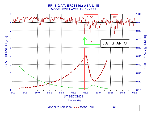
Figure 18. Model for layer thickness (green) and RRi(t) for an assumed potential temperature contrast (30 K) and wind vector contrast (18.2 [m/s per km]) cross the layer. The compression phase leads to rising RRi(t), adjusted so that RRi reaches 4.00 when CAT is observed. The model assumes a more rapid thickening caused by CAT, after which compression resumes (prior to a second CAT episode "1b").
During this initial compression phase, from 54.7 ks to 55.78 ks, for my assumed parameter values RRi begins with the value 0.19 (i.e., Ri = 5, which is typical for the undisturbed atmosphere) and reaches 4.00 at the time of CAT event "1a." The model then assumes that CAT causes a rapid thickening until RRi = 1.00 is reached (this is what theoretical calculations predict should happen). During this expansion phase I've assumed that with the onsset of CAT the layer starts to thicken by a factor 1.4 each 22 seconds (of flight). At 55.9 ks RRi has decreased to 1.00, at which time I stop the expansion and hold the thickness (and RRi) constant for about 1 minute. Then, I have modelled a resumption of compression, in order to account for CAT event "1b." This second compression phase has layer thickness decreasing by 13% of its current value every 22 seconds. In order to create more realism in this figure the plotted RRi is an exponential time-average, which willl be required to reduce stochastic measurement noise and other real-world effects. The specific time-averaging algorithm used is simply to average each new measurment of RRi with the previous average using weights 3% and 97%. This produces a time lag in RRi(t) of about 40 seconds, and this is judged a worthwhile price to pay for producing less noisy RRi(t) traces from real measurements (as will be seen shortly).
In this very simple model, once a layer thickness has been chosen, as well as potential temperature and wind vector contrasts across the layer, the only freedom allowed for adjustment is layer thickness versus time. I have chosen a simple sequence for layer thickness changes, consisting of a compression phase, an expansion phase following the onset of CAT, and another compression phase required by a second CAT event.
RRi Inferred from Measurements for CAT "1A" and "1B"
Now it is time to present RRi as inferred from the MTP measurements of lapse rate and the MMS measurement of temperature and wind along the flight path.

Figure 19. RRi before and after first CAT event. Turbulence intensity is shown "inverted" at the top. The two versions of RRi differ only in the time-averaging interval for RRi data having higher temporal resolution. The measurements used to calculate RRi in this figure is centered n the time that RRi is plotted; i.e., for the 2-minute average RRi trace a minute's worth of "future" measurements are used to calculate RRi.
This figure shows the result of calculating RRi using the algorithm described above.There's a clear pattern of increasing RRi building up to the first CAT event. During CAT "1a" RRi decreases, as it should according to theory. The RRi level reached during CAT is even consistent with theory, being approximatley 1.0. There's a brief resumption of the RRi build-up after CAT event "1a", but CAT event "1b" follows in quick succession and decreases RRi. Following CAT event "1b" RRi begins to build up again, but then decreases. CAT event "2" follows shortly after "1b" which tends to confuse the interpretation. The consistency of the observed pattern of RRi with CAT location with the pattern predicted by the vertical compression theory, constitutes compelling evidence that the vertical compression theory for CAT generation is the correct explanation for the two ER911102 CAT events "1a" and "1b."
The averages shown in this figure consist of 1-minute and 2-minute temporal averaging, centered on the time plotted. In other words, each RRi point makes use of as much measurement data for "future" times as it does for past times (measurements already made). This is an optimum way of analyzing data for the goal of gaining insight into the physical process under study, but it does not accurately represent what could be produced in real time in the aircraft. If this CAT warning algorithm were implemented aboard an aircraft it would be necessary to employ an algorithm that did not make use of "future" measurements. Consequently, I have performed a simulation that calculates RRi based on data available only up to the time for which RRi is displayed. The results of this simulation are shown in the next figure.

Figure 20. RRi versus time calculated using only data available up to the time for which RRi is calculated (simulating a real-time warning algorithm). As in the previous graph turbulence intensity is shown "inverted" at the top. If the RRi "heads up" warning threshold were set to 2.0, and if both the 1-minute and 2-minute RRi averages must exceed 2 to justify a "heads up" advisory, or yellow warning light, then an "advisory for CAT could have been issued 7 minutes before the start of CAT event #1a. If the actual warning threshold, or "red light warning," were based on RRi exceeding 2.5, then the actual warning of impending CAT would have been issued 3 minutes ahead of the event.
I have not yet established thresholds for CAT warnings, and CAT "heads up" advisories. In this figure I have indicated that RRi = 2.0 might serve well as a "heads up" advisory, while RRi = 2.5 could be used for the actual CAT warning. If these two thresholds were adopted, then the CAT event "1a" "heads up" advisory would have been issued 7 minutes before the encounter, and an actual CAT warning would have been issued 3.3 minutes before.
After CAT "1a" smooth flight resumes, for a couple minutes; but the RRi would have provided warning of more CAT. At second "CAT warning" would have been issued 3.0 minutes before the main feature of CAT event "1b". When two CAT events are as close together as 6.5 minutes, as the main parts of CAT "1a" and "1b" are, it may not be possible, and it may not be necessary, to issue distinct CAT warnigns. This is because it is customary to leave the seat belt sign "on" after a CAT encounter for several minutes before turning it "off" - based on the logic that a first CAT event is often correlated with subsequent ones. Therefore, I do not place mch significance on the performance, or lack of it, for CAT event "1b," given that it closely followed CAT "1a".
Comparison of RRi Compression Model with Measured RRi for CAT "1A" and "1B"
Out of curiosity, let's see how the model (Fig. 18) compares with the measurments.
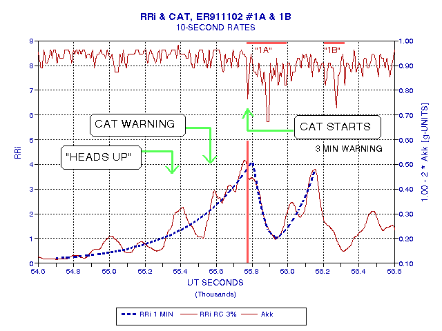
Figure 21. Comparison of modelled RRi(t) using a scenario for layer thickness changes (blue dashed trace) with measured RRi(t) (thin red trace). The agreement is excellent!
Well, OK - I did adjust the model presented in Fig. 15 so that it would fit the data! But, the point can nevertheless be made that a simple compression model for CAT generation can easily explain the measured RRi(t) pattern in relation to CAT encounters for this flight segment - which is one of the objectives of this web page.
RRi Envelope Concept
Let's return to thinking about the mesoscale forces driving compression and expansion, and ask what RRi(t) might look like if CAT did not occur when RRi reached the threshold value of 4.00. As explained in my overview of the compression theory for CAT generation, the synoptic scale produces alternations of vertical compression and expansion all the time, if only at small and usually insignificant levels most of the time. When the amplitude of these vertical compression/expansion oscillations becomes large, and when a layer is affected that contains wind shear, the ingredients are present for triggering CAT.

Figure 22. The black dashed trace is an "RRi envelope" that indicates how RRi(t) might have looked if CAT had not been triggered.
In this figure the flight time coverage has been extended to include CAT event "2." I have fitted a model for RRi (black dashed trace) that matches the measurement-inferred RRi trace where CAT is absent, and where CAT is present I have subjectively continued trends to make a continuous trace throughout. I call this an "RRi envelope" trace. Theory predicts that wherever the envelope RRi trace differs from the measured trace, i.e., wherever the measured trace is "deficient" in RRi, CAT has extracted energy from the wind field to homogenize the layer flown through. Clearly, there are three regions deficient in measured RRi, and they correspond to the three CAT encounters.
Notice that encounters "1a" and "1b" were produced by the first mesoscale compression, whereas the second mesoscale compression produced only one CAT encounter. The first mesoscale compression feature, extending from 54.6 ks to 56.7 ks, is much more expansive than the second compression feature, from 56.7 to 57.4 ks. These flight time widths correspond 500 km and 170 km along the ground track. Also, notice that for CAT event "2" there is little warning time. In fact, for CAT event "2" there would have been NO warning, unless the prudent strategy of relying upon CAT persistence were used to continue the warning of more CAT after the "1a" and "1b" encounters. The fact that CAT event "2" provided no warning is probably due to the three times smaller size of the mesoscale compression feature within which that event was triggered. Even flying "backwards" (from right to left) there would be a mere 1.0 minute warning (this is based on recalculating the "RC 3%" trace going in the backwards direction, consistent with flying backwards). Even this warning is lucky, and is due to the fact that the the CAT patch is off-center (with respect to the mesoscale compression feature). I conclude from this that some mesoscale compression events are going to be too small in horizontal extent to provide sufficient warning using the RRi trends of this study. This is an important result of the study, and it will beinteresting to see if this prediction is bourne out by future case studies.
Another interesting finding can be gleaned form Fig. 22. Flying backwards would have produced NO warning for CAT event "1b," but it would have provided adequate warning for event "1a." The backwarrds flight warning time for CAT event "1a" would have been 3.3 minutes. So far our score for forward flight and backward flight can be summarized in the following table, which assumes that warnings shall be issued whenever the "3% RC-time-averaged RRi trace" reaches 2.5:

Figure 23. IAC for the same time period of the previoius figure.
The large maountain waves at about 63 ks occur over 13.500-foot King's Peak, east of Salt Lake City, UT. I suggest that the mountain wave structure was compressed to the "breaking point" (when RRi exceded 4 for a sufficient time), causing the generation of CAT. If the CAT were generated by a "breaking wave," with an associated vertical expansion, the isentropes would have separated by large amounts just prior and during the CAT. Lapse rate (as use the term) would have decreased to -10 [K/km] just prior to the CAT, and just afterward.

Figure 24. Lapse rate, dT/dZp, and accelerometer activity, Akk, for the same period of the previous two figures.
The behavior of dT/dZp throughout this time period is "ambiguous," and I claim that the LR data, by itself, cannot be used to argue that CAT was generated by either the vertical compression mechanism or the wave breaking one. Before CAT event "1a" dT/dZp does show a decrease, but only to -1.5 [K/km] prior to CAT onset. My interpretation of the LR pattern is that there's an increase in stability up to 55.6 ks, and a decrease caused by previous CAT events in the region 55.6 to 55.79 ks causing dT/dZp to be low. The reason dT/dZp is not -10 [K/km] in this region and also where CAT is present, is that the MTP antenna pattern "beam" extends for several kilometers, and the volume fraction of CAT within the beam is approximately 1/2. For such a volume fraction of CAT and pre-CAT air, with LR values of -10 and +3 [K/km], respectively, the MTP would measure LR to be -3 [K/km]. But if just prior to CAT event "1a" the true value for dT/dZp is -10 [K/km], then one could argue that CAT event "1a" was caused by a wave that had produced an adiabatic layer just prior to breaking! This is just as valid an interpretation of the dT/dZp data, if the RRi data is not considered. But that's the key to understanding this event. The RRi data shows rising values up to the onset of CAT, and whereas this can be produced by a vertical compression of the layer of air that is destined to generate CAT, for the breaking wave scenario I don't think such a pattern would exist. (Comments from mesoscale wave experts are welcome.)
Aside from the ambiguity just discussed, it would be a good idea for the MTP to employ a slightly higher frequency, having a greater opacity, in order to produce a shorter "look distance," for then the MTP-measured dT/dZp would correspond more closely to the lapse rate at flight level. This change would be advisable for a CAT-intended MTP instrument.
CAT Event "7"
The RRi algorithm for predicting CAT will not work during ascents and descents, so we now proceed to the final CAT event for this flight, CAT event #"7."

Figure 25. RRi(t) for the level flight time period surrounding CAT event #7. The warning, based on RRi > 2.5, occurs 0.8 minutes before CAT onset (exceeds 0.20 g-units). The traces are the same as described in Fig. 17.
CAT event "7" is preceeded by a brief rise of RRi, and the tentative 2.5 threshold for warnings occurs only 49 seconds before the onset of CAT. Flying backwards through this region, and offsetting the RRi(t) lag appropriately, there would have been a CAT warning issued 6.7 mintues before the same CAT event started. I have not yet established a final protocol for expiring a CAT warning, so I cannot be sure I am justified in accepting this as a warning. Until I address this issue I will choose to accept this long a lead time as a warning.
The RRi feature centered on 60.6 ks is mysterious, since it reaches 4.00 without producing CAT. CAT event "7" occurs 16.7 minutes after the RRi feature, so it would have to score as a "false alarm." I will deal with false alarms at greater length in the next section, and I will devote a special web page to false alarms in general.

Figure 26. Lapse rate and accelerometer activity, Akk, for CAT event "7".
There is no evidence for compression just prior to this CAT event. The unusual rise at 61 ks occurs 8 minutes before CAT onset, and I doubt that it constitutes evidence for compression as the generator of this CAT. There also is no evidence that a breaking wave could have created the CAT, since the lapse rate did not move toward adiabatic before (or after) the CAT.

Figure 27. IAC for the same period of the previous figure. The aircraft's altitude is shown by a thick black trace.
There is no evidence in the isentropes of this figure that wave breaking could have caused CAT event "7."
Hit Rates and Warning Times Summarized
The following table summarizes warning times for the 4 level flight CAT encounters of this flight.
TABLE I
WARNING TIMES FOR LEVEL FLIGHT CAT EVENTS
| Flight Direction | CAT Event | Warning Time |
| Forward | "1A" | 3.3 Minutes |
| Forward | "1B" | 3.0 Minutes |
| Forward | "2" | 0.0 Minutes |
| Forward | "7" | 0.8 Minutes |
| Backwards | "1A" | 3.3 Minutes |
| Backwards | "1B" | 0.0 Minutes |
| Backwards | "2" | 1.0 Minutes |
| Backwards | "7" | 6.7 Minutes |
Warning time entries of 0.0 minutes is the same as a "miss." I shall arbitrarily adopt the requirement that minutes warning times must exceed 30 seconds to constitute a "hit." The last warning time entry would be 6.7 minutes, but since this is quite long, and since I have not yet established a limit for maximum warning times, I cannot now score it. Thus, we have 7 events that can be scored. Of these 7 events, we have 5 hits, and 2 misses.
False Alarms
The previous figure already featured a "false alarm" event from my tentative protocol for issuing CAT warnings from RRi. The RRi trace in the same figure reaches 2.5 on two other occasions, near the right side. At about 62.5 ks and 62.7 ks are two RRI features. However, these are artifacts produced by the ER-2's conducting an MMS box-calibration maneuver from 62.39 to beyond the right margin of the figure. During such a maneuver the plane rolls 20 degrees four times, completing a box pattern on the ground track. At the time of these observations the MTP instrument could not compensate for flgiht with this magnitudeof roll data, and the quality of MMS data is also compromised during such maneuvers. Thus, the two RRi features on the right are to be ignored.
There's a more serious problem with false alarms that occurs at the beginning of the flight, while flying over eastern Nevada.

Figure 28. RRi(t) for the beginning of flight ER911102, before the first CAT encounter. All the RRi features are "false alarms."
In this figure RRi exceeds the provisional warning level of 2.5 during most of the 18 minutes from 53.2 ks to 54.3 ks. An inspection of the 1-second resolution data indicates that the sepcific algorithm for deducing VWS can be contaminated by horizontal wind structure under certain conditions. During the false alarm period now in question the MTP lapse rates do not suggest that compression has occurred. The source of the high RRi values in Fig. 28 is due to high VWS values, which in turn might be due to correlations of horizontal wind with vertical motions. Perhaps this region consists of air that is undergoing correlated horizontal and vertical displacements from in an oscillating pattern that allows the algorithm for deducing VWS to be fooled by the horizontal oscillations. All data so far shown are for a 10-second time base. If a repeating oscillating motion is causing the artifacts of high RRi in the Fig. 21 data, then shoosing a different time base should produce different results.
When a 20-second time base is chosen for taking U, V and theta differences, and when inferred values for dU/dTH and dV/dTH are used to calculate RRi(t), indeed a different pattern for RRi(t) is produced for the time period covered by Fig. 28. The RRi's are worse! This is due to the presence of theta, U and V osciallations during this data interval with periods of predominantly 5 minutes, which is longer than the 10 and 20 second time bases. Therefore, the horizontal gradients produce a greater contamination of the inferred dU/dTH and dV/dTH estimates. Therefore, changing the time base will not improve the quality of RRi traces for this flight. At this point, there's just one thing left to try, which is pursued in the next section.
Multiple-Regression Solutions for U and V Depdendence Upon Time and Theta
Since U and V depend upon both horizontal location and altitude, an since the plane's in situ MMS data is probing both independent variables in a way that each is producing variations in U and V, it will be necessary to switch algorithms designed to minimize contamination effects of horizontal gradients of U and V. This, in fact, is essentially what I claim should be done in my patent, and described in some detail at a 1990 status report to the Navy. In that report I recommend the use of weighted averages of dU/dTH and dV/dTH, which employ weights that are low when dU/dt and dV/dt are high. In this section I will explore an alternative method for isolating the theta dependencies. I shall try using a multiple-regression analysis (also referred to as multivariate analysis) for deriving dU/dt and dU/dTH (and dV/dt and dV/dTH) simultaneously. Provided there is sufficient variation of both independent variables, and assuming they also vary in an uncorrelated manner, then this procedure should isolate the theta component of variation, leading to better quality values for dU/dTH and dV/dTH.
The equations for doing this have been worked out from first principles (I like understanding equations I use, and eschew lifting them from cookbooks), and code for this new procedure has been written. Details of this new algoritm can be found at Multiple-Regression Algorithm. Briefly, 31-second "chunks" of data is subjected to the following analysis: 1) multiple regression solutions are performed for the dependence of U and V upon both time and theta, 2) the square of the multiple correlation coefficients for the fits of U and V to these two independnet variables (i.e., R2) is calculated, 3) a "figure of merit" is calculated for later weighting purposes, which is the product of both correlation coefficent squares, and multiplied by the variance of theta, 4) the preceding procedure is repeated for all data, 5) a sliding 31-second weighted average is performed on the previous data base (by coincidence I chose 31 seconds for two steps in the overall procedure), resulting in weighted-average RRi(t).
Application of MR Algorithm to Current Flight Data
The next figure shows the RRi(t) results of using the Multiple-Regression analysis on the same raw data upon which the previous figure is based.

Figure 29. RRi(t) for the same time interval of the previous figure, but resulting from a multiple-regression analysis for assessing dU/dTH and dV/dTH.
In this figure the RRi(t) plot is a much "subdued" version of the previous one. Apparently the RR(t) in Fig. 28 was influenced by horizontal wind gradients, which presumably have been removed in this figure. Nevertheless, this figure shows the weighted-average RRi trace (black) exceeding 2.5 four times, and these would have to qualify as a set of "false alarms." Since the first three occasions of high RRi are close together in time, they probably will constitute one false alarm after I choose a protocol for issuing alarms.
What about the other false alarm case, represented by Fig. 25?

Figure 30. RRi(t) for the later portion of flight ER911102, surrounding the last CAT encounter.
Compared with Fig. 25, which covers the same time period but uses 10-second differences to deduce U and V dependenceis on TH, this trace of RRi(t) shows no false alarms. Apparently the earlier analysis was contaminated by wind horizontal gradients. The highest RRi feature occurs just before the CAT event "7" but provides a "warning" of only 1.5 minutes (after allowing for the fact that this figure plots RRi(t) at a time corresponding to the centroid f the data).
And now for CAT events 1a, 1b, and 2.

Figure 31. RRi(t) for the first CAT encounters, described above in Fig.'s 16 to 19. The dotted red trace is unaveraged 31-second multiple regression based RRi, and the thick black trace is a 31-second sliding weighted-average of RRi(t). CAT intensity is shown inverted, at the top, with a correction applied to measured peak-to-peak excursion to compensate for low sampling rate effects.
This figure is disappointing! Either RRi was really low throughout the CAT events, never reaching the warning threshold of 2.5, or the multi-regression solutions for U and V's dependence on horizontal location and theta partitions too much of the observed U and V fluctuations to the horizontal location independent variable, leaving too little for theta.
Review of Assumptions Relating to Partitioning Dependencies Between Two Independent Variables
Until now I have avoided a discussion of some subtleties concerning the way algorithms "partition" dependencies of U and V changes between the two independent variables "horizontal location (time)" and "theta." Since it appears that the two algorithms that have been tried so far are failing to properly partition dependcies, it is now worth a more detailed consideration of this challenge.
Consider the following "chunk" of data, covering

Figure 32. Detail of theta, U and V during a part of the flight immediately before CAT event "1a". The vertical time lines are 30 seconds apart, which assists in imagining boundaries for "chunks" of data upon which the multiple regression analysis is performed for deriving dependencies of U and V upon time and theta. Chunks "A" "B" and "C" are discussed in the text.
In this figure the eye can "see" correlations between theta and the U and V traces. For example, at "A" there is a clear correlation of a "hump" in theta with a corresponding "hump" in V. But at "B" and "C" there is a potential problem. Taken separately, which is what the multiple regression analysis does, the data in chunks "B" and "C" do NOT show a correlation between theta and U. Yet, the "eye" sees a correlation when the two chunks are considered as one. The MR analysis will find a least squares solution that partitions the bulk of correlation for U changes to "time" for both chunks "B" and "C."
The lesson, here, is that chunk sizes must be "compatible" with the duration of theta features. By "compatible" I mean the chunk sizes must be longer than the duration of theta features. On the other hand, chunk length must also be shorter than the decorrelation time for horizontal gradients, or the decorrelation time for U and V with theta. These decorrelation times are unknown, a priori, so I have tried to err on the side of short chunk lengths. But given the shortcomings of 30-second chunk lengths, seen in Fig. 32, I think it is time to try a longer chunk length for the MR analysis.
In retrospec I now understand that use of the 10-second base for interpreting differences in terms of theta dependencies only will always lead to RRi values higher than true; they will produce an RRi(t) treace that is an upper limit to true RRi(t) because none of the changes in U or V are attributed to horizontal gradients. The 31-second MR analysis, however, will have the opposite bias; it will produce an RRi(t) trace that is the lower limit of true RRi(t) because too much of the U and V changes are attributed to horizontal gradients whenever chunk length is too short. By increasing chunk length, from 31-seconds to 61 seconds, for example, the MR analysis should produce an RRi(t) trace that is closer to true.
Explorations of Other Chunk Sizes Using MR Analayses
I will save the reader a lot of grief by simply summarizing what I did. Anyone wanting to see speciic graphs of results may request them. I have several dozen that were used to produce this summary.
Briefly, the multiple regression analyses did NOT work! I evaluated longer chunk lengths (61, 91 and 121 seconds) and shorter one (21 and 11 seconds). The "best" chunk length among those tried was 31 seconds (Fig. 30), but differences were small.
Then I tried single regression analyses. By single regression I mean performing a linear least squares regression analysis in which U (and V) are the dependent variable, and theta is the sole indepenent variable, for data chunks. Doing this removes any possibility of horizontal gradients "stealing" correlation from theta. As expected, the dependence of U (and V) upon theta increased (with respect to the MR results). The single regression RRi(t) plots were indeed "better" than the multiple regression ones, and the best chunk length was 21 seconds (again, with small differences versus chunk length). However, they were not as good as the RRi(t) plots produced using the 10-second difference algorithm. The single regression 30-second weighted averages for RRi reached only 2.5 prior to the CAT event "1a", and the unaveraged RRi reached 7.5. Also, the false alarm problem for the section of data preceding the first CAT encounter was improved. However, the overall reduced RRi prior and following CAT events '1a", "1b" and "2", compared to those obtained using the 10-second difference method, argue for a reconsideration of the approach taken in deriving VWS.
Taking Stock of MR, SR, and Difference Methods for Evaluating VWS
Recall that the reason for trying the multiple regression (MR) algorithm was to remove horizontal gradient contamination of VWS in order to avoid false alarms. The assumption driving this strategy change was that horizontal gradients existed at 10-second timescales (which translates to 2.4 km distance scales). I had assumed that the appropriate RRi levels surrounding the CAT events was evidence that horizontal gradients didn't exist at these short distance scales for those times, but that such horizontal gradients did occasionally exist elsewhere. Specifically, I suspected that they existed in the "false alarm region" (53 to 54 ks), 30 minutes before the first CAT events (Fig. 28). But the presence of large RRi in the "false alarm region" when using the MR method (Fig. 29), for even the long chunk lengths, shows that RRi and VWS are indeed large there. In other words, the 10-second difference method was CORRECTLY reporting large RRi in the false alarm region.
The values for RRi using the MR and SR methods is lower than when the difference method is used. Compared with the 10-second difference method, the SR (single regression) values for VWS are at 70%, and for the MR (multiple regression) method VWS values are at 48%. This is a curious finding. I do not understand why the SR and difference methods produce different values for VWS for chunks of air 1.5 km across (traversed in 11 seconds). Perhaps this is due, somehow, to a violation of hydrostatic equilibrium of mesoscale waves. I also do not understand why lapse rate does not show evidence for compression in the "false alarm region" (53 to 54 ks, Fig. 14). Referring to the MTP lapse rate plot of Fig. 14, compression begins at 53.8 ks and continues until 55.2 ks. It is at this time that RRi begins to rise in a significant way (Fig. 20). Perhaps earlier CAT events in the pre-CAT region (from 55.2 to CAT event "1a") produced a vertical mixing of air that erased the lapse rate signature for compression. But then why does VWS build up throughout this pre-CAT region.
I confess to an incomplete understanding of what's happening! I suspect that someone with meteorlogy credentials is needed to sort out some of these mysterious effects. My goal for the present effort, being documented at this web site, is to assess a method for predicting CAT. This goal does not embrace a full interpretation of the observations used to make the CAT predictions - as much as I would like to do that. I would be going astray too far were I to devote more time trying to reconcile every observation that does not readily render itself compatible with the compression hypothesis for CAT generation. For now, I must leave these troubling anomalies with VWS differences and lapse rate patterns that don't completely match my simple version of the compression hypothesis, and hope that someone more qualified will rise to the challenge. But this invitation will only become interesting if the version of RRi used in this analysis, flawed as it may be, is predictive of CAT - which is the task to which I now return.
At this time there seems to be no reason to abandon the difference method for inferring VWS (and RRi). It was not flawed because it produced large RRi where CAT was not encountered, since the other methods also produced large RRi there; so it probably was not flawed (in this way) during the CAT region, where it produced RRi values in perfect agreement with theory. This state of affairs constitutes both "good news" and "bad news" for the task of predicting CAT. The "good news" is that a simple difference method might predict CAT, but the "bad news" is that it may also produce false alarms.
I have not yet analyzed enough data to address the false alarm problem. However, code now in hand should enable large amounts of flight data to be analyzed with a much smaller user investment of time. Therefore, I will defer the task of assessing the false alarm problem to a later time, when I can address it in a more systematic way (i.e., choosing flights reported to be "smooth" etc).
Additional Difference Method Analyses
Since the difference method appears to have merit, and does not suffer noticeably from horizontal gradient contamination, it is worth exploring a range of values for some of the parameters whose values were chosen with a subjective intuition. Specifically, the "difference span" interval of 10 seconds, has not been optimized. It is possible that a different choice of a difference span interval, hereafter referred to as DD, might provide either less noisy VWS and RRI values or might be less vulnerable to horizontal gradient contamination.
A range of DD values (difference span) were evaluated (3, 5, 7, 10, 15, 20, 25 and 30 seconds), and by coincidence DD = 10 seconds is the optimum. Larger DD values produce very similar RRi(t) for most time periods, whereas shorter values produce smaller RRi (for reasons I don't understand). For example, for the time interval 54900 to 55700 RRi based on DD = 25 seconds is plotted versus RRi based on 10 seconds, shown in hte next figure.

Figure 33. Scatter plot of RRi based on DD = 25 seconds versus RRi based on DD = 10 seconds. A least sqauares fit line shows that the 25- second RRi values are only 8% larger, on average, than the 10-second RRi values.
In this scatter diagram if horizontal gradients were present they would RAISE the values of the 25-second RRi estimates in relation to the 10-second RRi's. In fact, if the RRi were estimates were due exclusively to horizontal contamination the slope of the fitted line would be 2.50 (=25/10), instead of the observed 1.08.
The slopes for all DD values evaluated (for the specified time interval) is shown in the next figure.

Figure 34. Amplitude of RRi versus "Difference Span" DD, for the time interval 54900 - 55700 utsec.
The small RRi values for DD smaller than 10 seconds may be caused by an insufficient range of theta sampling for short timescales. For difference spans of 10 seconds and longer the range of theta sampled apparently is sufficient to establish a correlation between U and theta (and V and theta), allowing for VWS to be adequately determined. From this figure it is concluded that DD = 10 seconds is optimum for evaluating VWS (and RRi).
It should be noted that the horizontal gradients in other regions may be larger, and may introduce falsely high values for VWS (and RRi) for timescales DD < 30 seconds. Therefore, in order to reduce the chance of horizontal gradient contamination using the DD technique for deriving VWS, it is important to keep DD as short as possible. Use of DD = 10 seconds will be provisionally adopted.
Concluding Remarks for Flight ER911102
I am adopting the difference method for determining the correlation of U (and V) with theta, and for this flight I shall adopt DD = 10 seconds. Therefore, the RRi(t) plots in Fig.'s 19 through 22 will be accepted. Table I has not been superceded, so we still have a "score" of 5 hits and 2 misses for the 7 CAT encounters that can be scored. The median warning time is 3.0 minutes, and the average is 2.3 minutes.
The exercize of trying out two alternative methods for estimating the correlation of U (and V) with potential temperature (theta) was instructive. The "single regression" method (SR method) produced correlations (i.e., VWS) that were 70% of those produced by the "difference span" method (DD method). The "multiple regression" method (MR method) produced correlations that were, in turn, 70% of those produced by the SR method, i.e., they were 48% of the DD correlations. Whereas the SR method allowed theta to absorb the entirety of correlation, leaving none for horizontal gradients, the MR method allowed for the simultaneous correlation of U and V with both theta and horizontal gradient. I do not completley understand these differences in correlation amplitude, but I suspect they are somehow related to the fact that small "bobbing motions" of mesoscale-sized chunks of air do not preserve their horizozntal wind vector in a conserved manner. Theta will be conserved, so any discrepancies with my simple model, which require that isotachs and isentropes follow the bobbing motions, should be attributable to the breakdown in the isotach assumption.
I have adopted the DD method for correlating U and V with theta because this method produces RRi results that are in very good agreement with theory. I could just as well have adopted the SR (or MR) method. If this were done, however, I would have to adopt RRi thresholds for CAT that were 1/2 (and 1/4) of the values I have adopted for use with the DD method. There is nothing in the present flight's data to give preference to any of these three methods, since they all showed rising RRi before CAT, and they all showed RRi features where CAT did not exist. If future flights indicate that the DR, or MR, method is superior to the DD method, I may switch to the superior performing method.
The issue of false alarms will be an important issue to address, but I prefer to do this at a later stage of this work. Flights identified as "smooth" by the pilots should serve as the best data source for evaluating false alarm rates.
This, for now, completes my analysis of flight ER911102. I am ready to proceed with a DD analysis of the rest of the flights identified for use with this task.
____________________________________________________________________
This site opened: July 26, 2000. Last Update: September 20, 2000