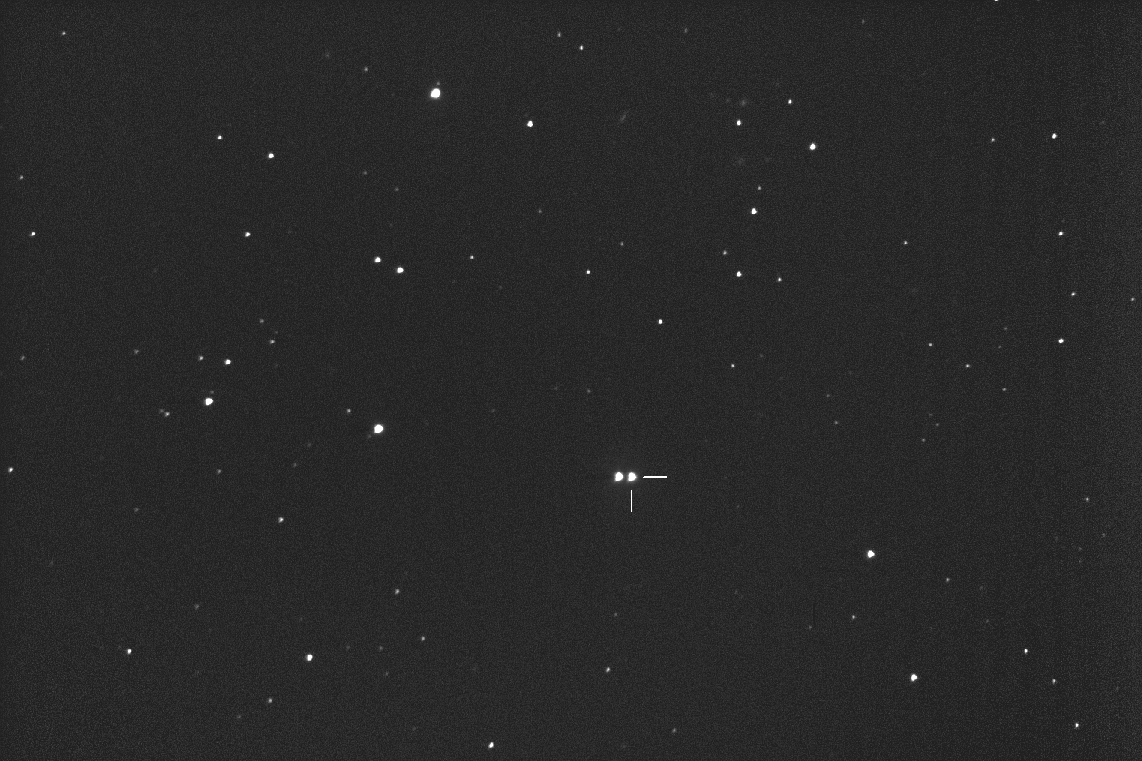
Figure 1. Star field surrounding HD 80606 (indicated) and it's orbital companion star, HD 80607 (to its left). FOV = 31 x 21 'arc, north up, east left. FWHM ~ 4.2 "arc.
This web page describes an evalutaion of several observing and image analysis strategies for the exoplanet HD 80606b. The usual procedures of maintaining sharp focus and using a photometry aperture radius ~4 times FWHM was compared to an alternative observing strategy, defocusing, which for my telescope system produced superior results. This is due in part to the brightness of HD 80606 and also to the fact that its equally bright orbital companion, HD 80607, is located only 20 "arc away.
Introduction
HD 80606 has an exoplanet that orbits with a 111-day period in a very eccentric orbit (0.93). The orbit is inclined close to 90 degrees because when it is behind the star it undergoes a "secondary" transit, as observed with the Spitzer Space Telescope by Laughlin et al (2009). It is not known if the planet transits in front of the star, for a primary transit, because that part of its orbit is much farther from the star. An opportunity for observing a possible primary transit exists on Feb 13/14 UT of 2009. This web page has been created for offering suggestions on the best strategy for conducting these observations and for processing the images to produce a light curve.
Hardware
My telescope is a 11-inch aperture Celestron (CPC1100) mounted on an equatorial
wedge. I use a focal reducer and SBIG AO-7 image stabilizer in front of a
SBIG ST-8XE CCD camera. The AO-7 employs a tip/tilt mirror that can be operated
at several Hz, and when mirror motion exceeds a user-specified limit a correcting
nudge signal is sent to the telescope drive motors. The polar axis has been
aligned to the north celestial pole with an accuracy of ~2 'arc. This assures
that when the AO-7 keeps an autoguided star fixed to a pixel location on the
autoguider chip the star field does not rotate about that star and simultaneously
move the star field across the main CCD chip. This arrangement assures that
the star field is fixed with respect to the CCD pixel field to within a few
pixels during the course of a many hour observing session. The image scale
is 1.21 "arc/pixel, and the FOV is 31 x 21 'arc. I use a wireless focuser
(Craycroft type) for adjusting the position of the optical back-end (the mirror
is not moved). MaxIm DL 5.03 is used to control the telescope, wireless focuser,
AO-7 and CCD camera.
Each observer's hardware is different, and atmospheric seeing is different
each night, so the following is presented with the purpose of illustrating
concepts that can be used to guide observers in choosing optimum observing
and image analysis strategies.
Review of Usual Strategy for Exoplanet Transit Light Curves
Normally, transiting exoplanet light curves are produced using sharply-focused
images and a photometry aperture radius ~ 4 x FWHM. Slightly smaller and larger
photometry apertures can sometimes produce small improvements (e.g., ApertureRadius/FWHM
within range 3 to 5). However, when a star is close to the target star it
may not be possbile to employ this standard aperture setting. Exposure times
are chosen that yield maximum counts for stars of interest that are slightly
less than the linearity limit (52,000 counts for my CCD) at times of best
atmospheric seeing. Here's an image of the HD 80606 star field.
Figure 1. Star field surrounding HD 80606 (indicated) and it's
orbital companion star, HD 80607 (to its left). FOV = 31 x 21 'arc, north
up, east left. FWHM ~ 4.2 "arc.
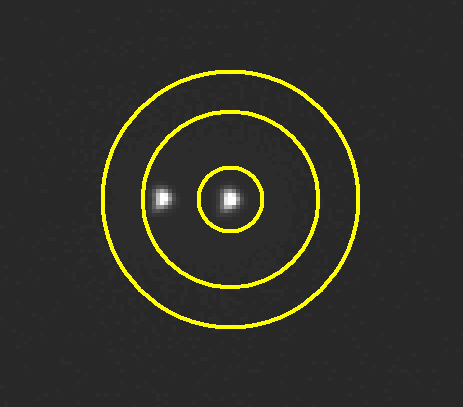
Figure 2. Zoom of previous image showing a photometry aperture
centered on HD 80606 and HD 80607 20.5 "arc to the east. FOV = 9.3 x 8.2 'arc.
The aperture radius is 9.7 "arc (8 pixels), which is ~2 x FWHM for most images
of this observing session.
Fig. 2 gives the impression that it is possible to employ a small photometry
aperture for stars as close as 20.5 "arc (17 pixels). However, the brightness/contrast
setting for this image gives a false impression of each star's PSF (point-spread
function). Here's a different brightness/contrast choice.
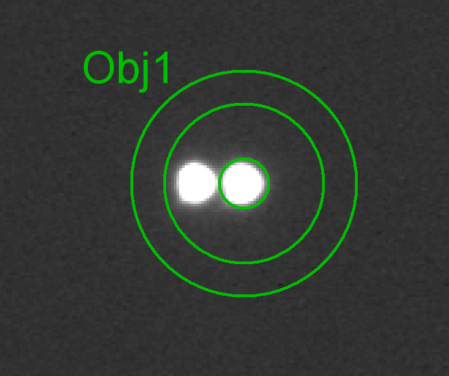
Figure 3. Zoom showing a photometry aperture radius of 10.9
"arc (9 pixels), which places a boundary of the signal aperture half-way between
the two stars.
Fig. 3 shows a signal aperture choice that should be least affected by
atmospheric seeing changes that cause the PSF of the nearby star, HD 80607,
to "spill over" into the signal aperture while the same seeing change causes
the target star's PSF to "spill out" of the signal aperture by approximately
the same amount. For this observing session, and for exposure times of 30
seconds (the longest exposure time that still prevents saturation), PSFs have
FWHM values that are typically 4.5 "arc. This aperture corresponds to the
ratio ApertureRadius / FWHM = 2.0, which is not within the customary
3 to 5 range where best results are usually obtained. This suggests that
using this aperture it may not be possible to obtain a high precision light
curve.
Three Strategy Candidates
In anticipation of problems with the usual observing strategies I note three approaches to observing HD 80606:
1) Choose a photometry aperture radius of 1/2 the separation
of HD 80606 and HD 80607 (i.e., 1/2 of 20.5 "arc ~ 10 "arc), and hope this
is adequate (e.g., Fig.3),
2) Choose a photometry aperture that includes both stars,
and accept the added noise from the larger number of pixels within the signal
aperture (e.g., Fig. 8, below), and
3) Defocus all images the same amount and use a large
photometry aperture to include both stars (Fig. 10, below).
Note that a defocused image can accomodate a much longer exposure time
than a sharply focused image, thus improving the duty cycle (defined as "time
exposing an image divided by interval between images"). For example, one of
my image sets had an exposure time of 10 seconds (sharply focused) and the
defocused images had an exposure itme of 60 seconds. Since my overhead is
12 seconds (8 seconds for image download and 4 seconds for the AO-7 to adjust
tracking), the corresponding duty cycles are 45% and 83%. The number of photons
collected per unit time are in the same ratio, 45 and 83, so the defocused
image set yields almost twice as many photons per unit observing time as
the 10-second image set. Duty cycle advantages for defocusing are greater
for bright stars since brightness calls for short exposure times for sharply
focused images (to avoid saturation).
Strategy 1: Sharp focus, small aperture
This strategy is as close to what normally is done as possible; only the
photometry aperture is smaller than normal because of the nearby star HD 80607.
The exposure time was 30 seconds, which kept all stars in the FOV just below
saturation. The following image shows my choice for reference stars.
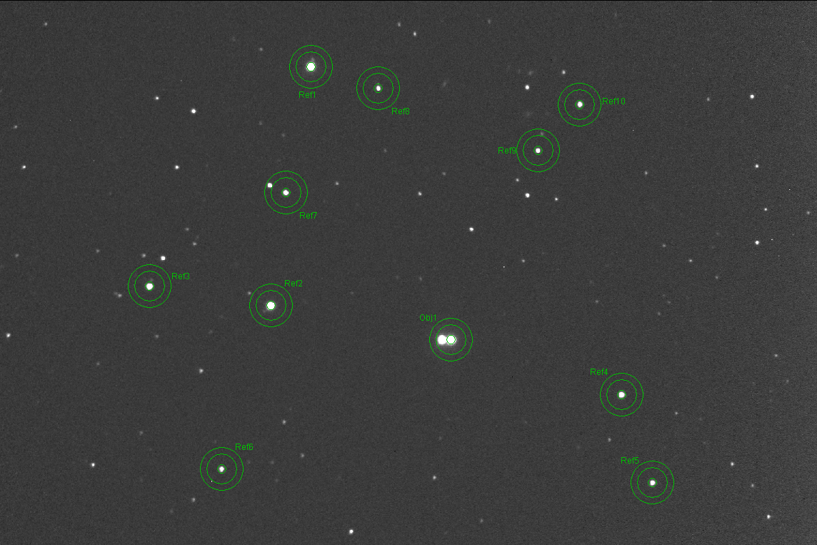
Figure 4. Sharply focused and 30-second exposure star field with
10 reference stars indicated.
This strategy was employed for an hour, and the next figure shows processed
light curve.
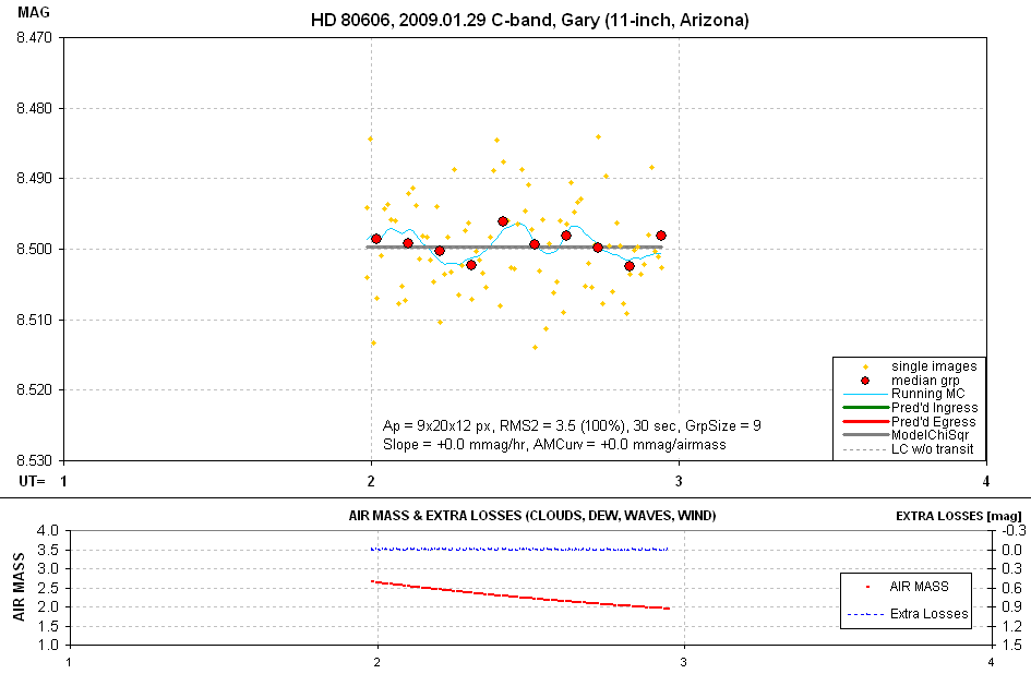
Figure 5. Light curve of HD 80606 for the sharply focused, 30-second
exposure image set.
The single image RMS is equivalent to a normalized 2-minute exposure having
RMS = 3.5 mmag per image. Taking the 71% duty cycle into account these data
correspond to achieving a precision of 4.15 mmag per 2 minutes of observing
time. This is greater than I normally achieve (edven for 11th magnitude stars),
so this appears to support my expectation that the precision suffers from
having to use ApertureRadius/FWHM = 2 instead of the normally optimum 4.
It occured to me that I could improve precision if shaper images could
be achieved. One way to improve sharpness is to use shorter exposures. So
I took another hour of 10-second exposures.
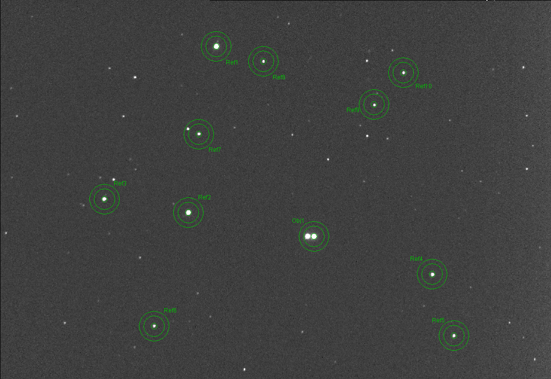
Figure 6. Shorter exposure image (10 seconds instead of 30 seconds)
showing the same photometry aperture setting as before (9x20x12 pixels).
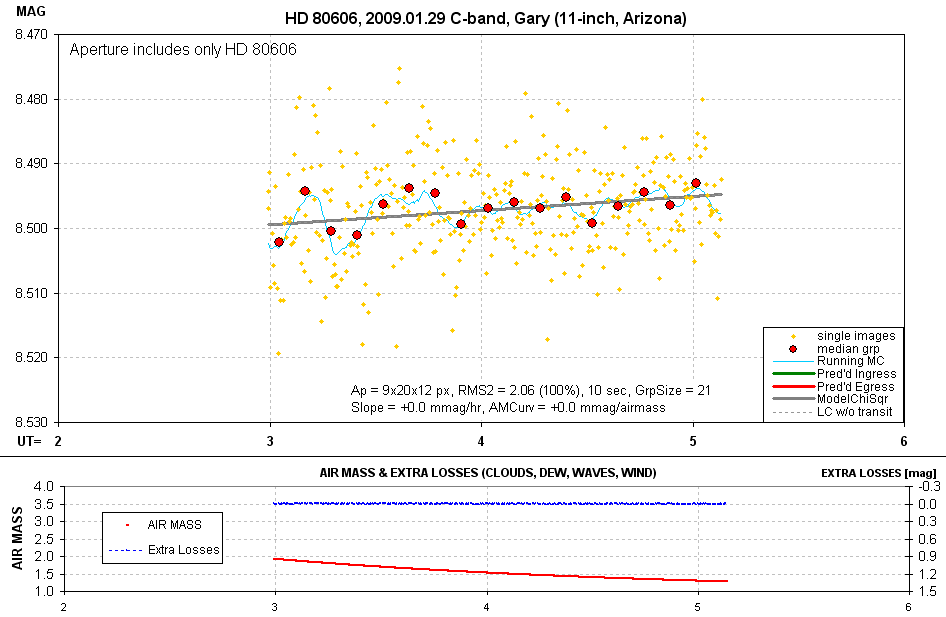
Figure 7. Light curve for above set of images.
The precision per image, normalized to a 2-minute exposure, is 2.06 mmag,
which is the kind of improvement that what I was hoping for. However, 10-second
imaging has a duty cycle of 45%, and adjusting for this yields a precision
of 3.07 mmag per 2 minutes of observing time. This is still significantly
better than the precision of the 4.15 mmag per 2 minutes of observing time
calculated from the 30-second exposure image set.
Strategy 2: Sharp focus, large aperture
The 10-second images were processed using an aperture that included the
flux fromboth HD 80606 and HD 80607, as shown in the next image.
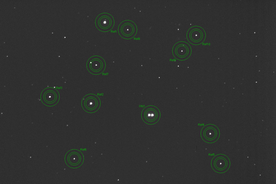
Figure 8. Using a large aperture for the same images as in the
previous analysis (10-second exposures). Aperture dimensions are 28x8x16 pixels.
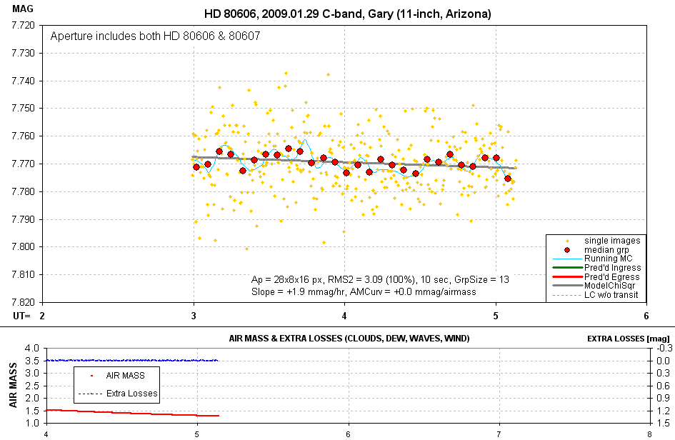
Figure 9. Light curve from 10-second, sharply focused images
but using a large photometry aperture that includes both stars.
The large aperture led to a worsened RMS per image. After correcting for
duty cycle the precision is 4.61 mmag per 2-minutes of observing time.
Strategy 3: Defocused, large aperture
The following defocused image is from a 1-hour observing session immediately
following the previous image set.
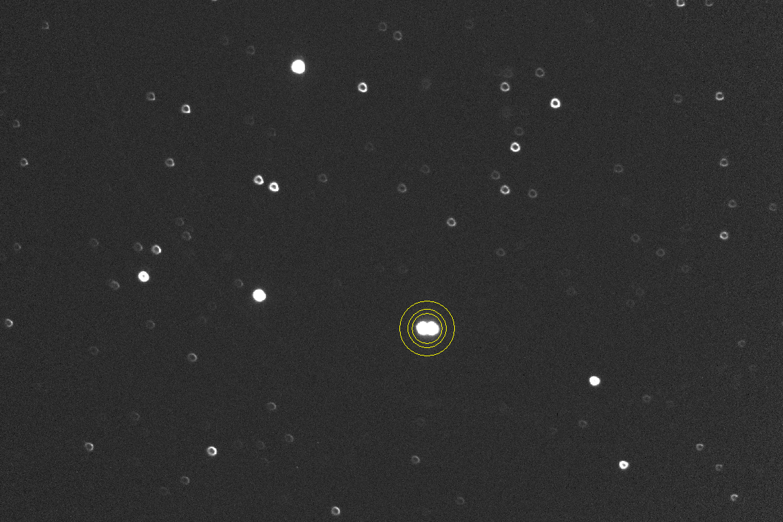
Figure 10. Defocused image showing the same large photometry aperture
used with the sharply focused images. Exposure time is 60 seconds.
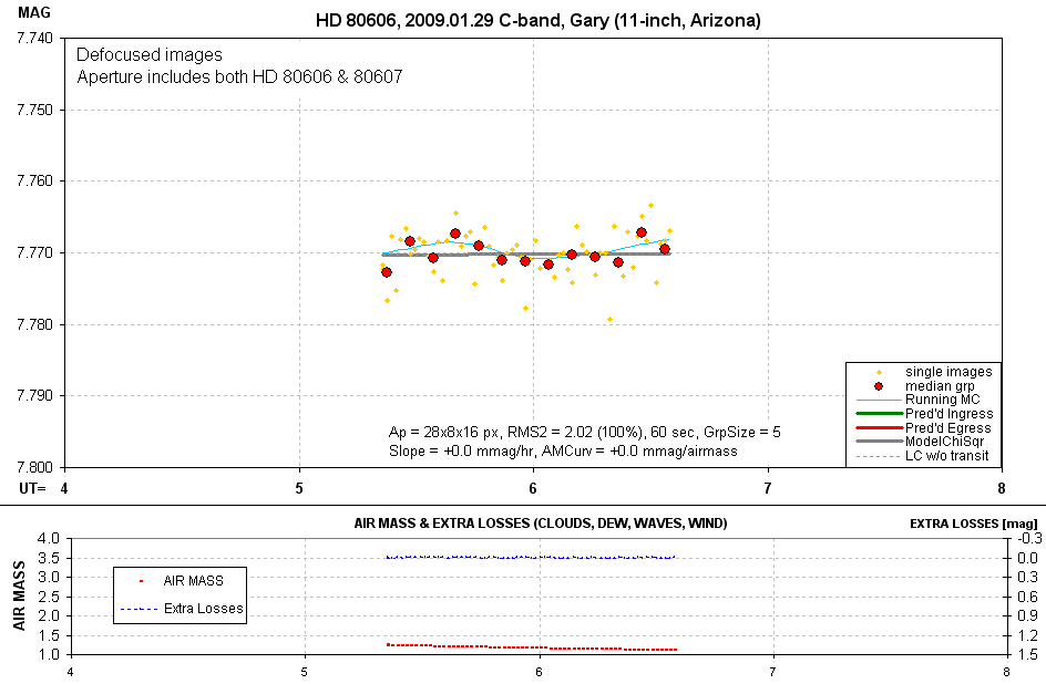
Figure 11. Light curve from defocused images and large photometry aperture
that included both stars.
The 2-minute equivalent RMS per image is 2.02 mmag, and correcting for
duty cycle yields 2.22 mmag per 2 minutes of observing time. This is better
than any of the other observing and analysis strategies.
Why?
I used to think that the only reason for defocusing was to improve duty
cycle. But compare the "sharply focused image set with large aperture" with
"defocused image set with large aperture" (same apertures), and the RMS per
2-minute equivalent image, unadjusted for duty cycle, is better for the defocused
image than for the sharp image. The two precisions are 3.09 mmag per image
and 2.02 mmag per image. Since duty cycle has nothing to do with these two
precision calculations there's something going on that has to do with the
spreading out of where photo-electrons are produced.
Could it be that when most of the star's photo-electrons originate from
only a few pixels that the readout noise per pixel, or the thermal noise per
pixel, has a greater percentage effect on the total flux than when many pixels
are involved? When most of the photo-electrons come from just a few pixels
could small errors in the flat field contribute a greater error in the total
flux than when these flat field errors are averaged-out over more pixels?
Could someone help me understnad this?
Conclusion
It's not necessary to understand why a defocused observing session produces
better results than a sharply-focused observing session, for a specific target,
when all we want to know is how to achieve the best quality light curve. I
concluse that for my hardware, and this target, and the atmospheric seeing
that existed for this test, it is better to observe defocused!
Since other observers will have different image scales and different atmospheric
seeing, if the best quality light curve is to be achieved on February 13/14
it will be necessary for each observer to perform a simple version of what
I described on this web page.
____________________________________________________________________
WebMaster: B.
Gary.
Nothing on this web
page is copyrighted. This site opened: 2009.01.30. Last Update: 2009.01.30