Bruce L. Gary; Hereford, AZ; 2004.11.22

ABSTRACT

This web page suggests that remote sensing systems for such things as "altitude temperature profiles" be evaluated using an alternative to the customary plot of SE accuracy versus altitude. A new measure for performance is suggested in which each retrieved temperature profile is compared with a "kernel layer averaged temperature profile," and a set of these profile differences is used to derive SE versus altitude. The virtue of this new performance measure is that it should quickly show the user of the remote sensor whether its performance is close to optimum. Specifically, it should provide a simpler way to assess the need for improving calibration, retrieval stratification procedures, instrument stability and radiometer stochastic noise level. [More text coming] 

Links Internal to this Web Page

    Introduction
    Averaging Kernel Basics
    Typical RMS Within Averaging Kernel Layers
    Example of Expected Performance
    Clever Retrieval Algorithms
      
   

Introduction

For a remote sensing system that retrieves "altitude temperature profiles" it is customary to describe performance accuracy with a plot of SE uncertainty versus altitude. In order to improve performance several things can be done: 1) radiometer noise figure can be reduced (to lower stochastic uncertainties), 2) systematic errors can be reduced by performing better calibrations, 3) more observables can be measured (either more frequenceies or more elevation angles), and 4) more sophisticated retrieved procedures can be developed. Each of these improvement possibilities requires a great amount of effort. These is a tendency to think that if only a better radiometer (with a lower noise figure) could be bought, or if only more frequencies or elevation angles could be measured during an observing cycle, or if only all calibrations could be established with great accuracy, the resultant profiles of SE performance could be improved to arbitrarily small values (high accuracy).

Alas, there is a limit to what can be achieved by all these strategies, and it is a fundamental limit imposed by the physics of remote sensing. It is my opinion that the performance levels currently achieved by Dr. M. J. Mahoney, using the JPL Microwave Temperature Profilers, is very close to this ultimate performance. The fundamental performance limit has to do with "averaging kernels." This web page attempts to show typical limits using a "best possible" averaging kernel.

Averaging Kernel Basics

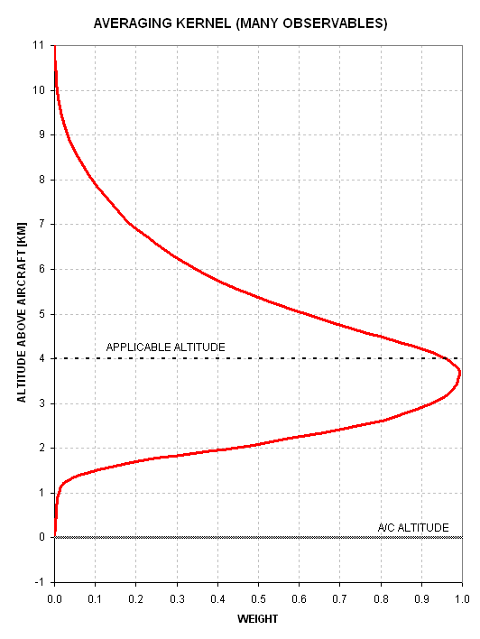
An averaging kernel is obtained by multiplying weighting functions by an appropriate set of retrieval coefficients. Each weighting function starts with a value of 1.00 at flight level and decreases exponentially (approximately) with an e-folding altitude scale height that is the reciprocal of the local atmosphere's absorption ccoefficient [Nepers/km]. It is desireable to use retrieval coefficients that produce an averaging kernel that is "narrow." The following illustrates a best possible (narrowest possible) averaging kernel.

Figure 1. Averaging kernel (red) obtained using at least a dozen observables with low noise. The "applicable altitude" for the averaging kernel is at an altitude 4 km above flight level.
 
This figure provides insight into what is actually measured when retrieving air temperature at 4 km. The retrieved air temperature is actually the weighted average of air temperature, where the averaging kernel is the weighting function. In other words, it is approximately correct to state that when the MTP retrieves an air temperature for an altitude 4 km above flight level the value that is retrieved is actually a layer average, and the layer in question extends from about 2 km to 5.5 km (using "full-width, half-maximum" to describe the layer).

A profile of retrieved air temperature is built from a series of such layer average results. For example, the following figure shows the relationship between two averaging kernels.

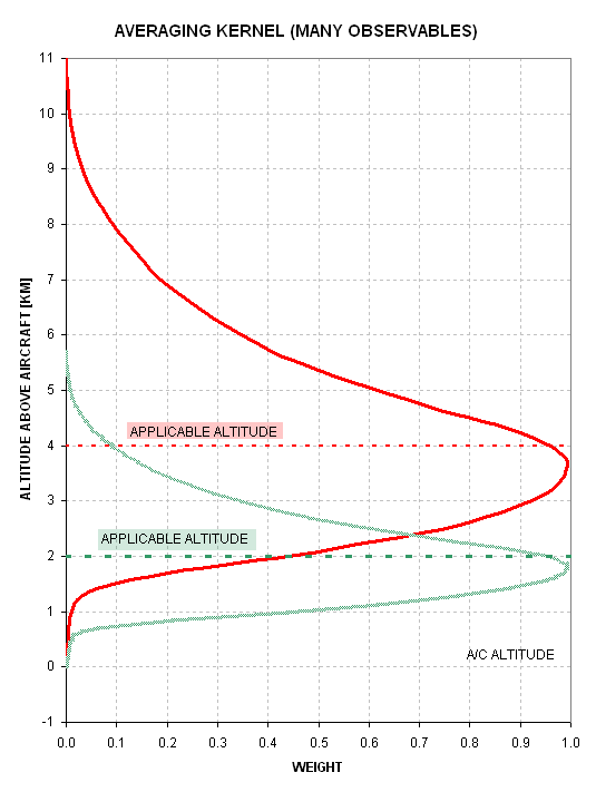
 Figure 2. Two averaging kernels, one for retrieved air temperature at 4 km above flight altitude (red) and another for 2 km (green).

The 2 km averaging kernel is narrower than that for 4 km, and this suggests that accuracy should be best close to flight level (which it always is).

Clearly, the reason narrower averaging kernels produce more accurate results is that the air temperature at the applicable altitude is more likely to be the same as the layer average. It may be possible to achieve any desired accuracy for a layer average temperature, but SE performance is rarely presented this way. For the person who wants to know how well a remote sensing system is performing, for the purpose of deciding whether additional improvements should be attempted, SE performance shouldn't be derived by comparing retrieved temperature profiles with actual temperature profiles, as is customarily done; instead, SE performance should be derived by comparing retrieved temperature profiles with layer average temperature profiles.

It will be useful to give a name to this new SE performance. Allow me to suggest the name: Kernel Temperature Performance, or KTP.

Think of KTP as an plot, versus altitude, of RMS difference between "retrieved air temperature" and "kernel layer averaged temperature." A KTP plot can be expected to be "flat"  versus altitude, with possibly a value of < 1.0 K throughout the range of applicable altitudes associated with the retrieved profile. This should be the case for all geographic and seasonal regimes, provided attention is given to the use of optimal retrieval procedures (stratified retrieval coefficients, etc) for all regimes. A plot of KTP should therefore be useful in assessing when additional attention should be given to a specific mission's MTP calibration or retrieval analysis.

Typical RMS Within Averaging Kernal Layer

In this section I want to establish an appreciation for the importance of the difference between air temperature at an altitude and the "averaging kernel layer average temperature." This difference will grow with averaging kernel layer thickness. I will use the following abbreviations:

    W = full-width/half-power layer thickness, using the "best possible" averaging kernel shape (given above),
    Tw = layer-average temperature using an averaging kernel with width W

Since the averaging kernel shape is assymetrical about the applicable altitude, with a long "tail" on the far side of the applicable altitude, it will be necessary to specify whether the shape is the same as shown in the figures above (for retrieved air temperature above flight level) or reversed (for below flight level). In deriving a plot of Tw versus altitude with respect to flight altitude the appropriate shapes will be used, i.e., reversal will occur for below flight level and the shape will be "scaled" for the applicable altitude to flight level distance. I note here that for applicable altitudes far from flight level the best possible averaging kernel shape cannot be achieved (for the far side) since there are no observables to sharpen the far side of the averaging kernel. Thus, by using one shape, simply scaled for distance and reversed for the below flight level regime, the calculated difference of T(z) and Tw(z) will be an under-estimate (on average) of the difference profile.

For a specific radiosonde (RAOB) and specific flight altitude I shall calculate dTw(z), which is simply Tw(z) - T(z). When this is done for many RAOBs it iwll be possible to calculate RMS(z), or the RMS deviation of the many dTw(z) profiles. RMS(z) for other aircraft flight levels can be calculated, but since the bulk of an aircraft's time is spent at a typical cruise altitude I will restrict my calculations to these most relevant altitudes. For the DC-8 this median altitude is ~11.4 km, and for the ER-2 it is ~19.4 km. Hence, I will generate only two RMS(z) traces. These RMS(z) traces will represent the best possible retrieved temperature profile performance that can be achieved using an MTP.

Note that a trace of RMS(z) for the DC-8 aircraft placed at 11.4 km will be valid only for the region and season associated with the RAOBs used. Many sets of "best possible" RMS(z) performance traces could be generated, but that is not my purpose here. I will choose just one region and season (one mission for which I have the required archive), and use it to demonstrate the central concept of this web page.

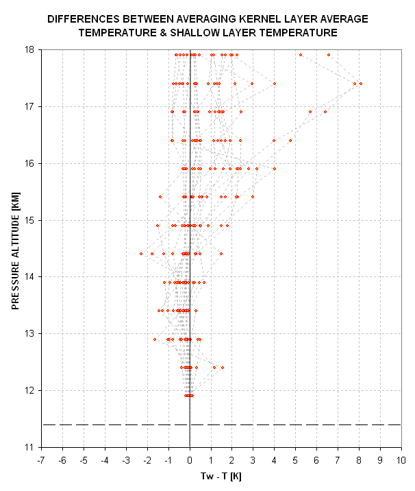
 Figure 3. Example of difference between Tw(z) and T(z) for 17 RAOBs from the TOTE/VOTE mission. Data for only altitudes above flight level (11.4 km) are shown.

In this figure there is a trend with altitude for the individual comparisons of retrieved versus RAOB temperature. This is caused by the persistence of a characteristic shape of actual T(z). For example, two of the traces in this figure correspond to Hawaii soundings, where the tropopause is always at 16 or 17 km. An averaging kernel with applicable altitudes hear these altitudes can be expected to produce Tw that is always too high compared with T. Effects such as this one can be removed by an empirical offset adjustment, EOA(z), that should be applied to all retrieved profiles as a final adjustment. (This was done for the measured RMS(z) performance used for TOTE/VOTE data, below.)

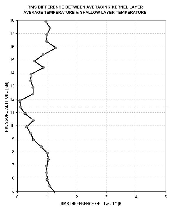
 Figure 4. Example of RMS difference between Tw(z) and T(z) for 17 RAOBs from the TOTE/VOTE mission.

What is the averaging kernel for flight level? It's not a delta function, as implied by the procedure used for other altitudes. The "averaging kernel" to be used for flight level should be based on the finitie beamwidth function for the three channels used in the DC-8 MTP. The applicable ranges for these channels are ~2.5, ~1.3 and ~0.6 km, and the 7.7 degree HPBW function produces a source function versus altitude shown in the next figure.

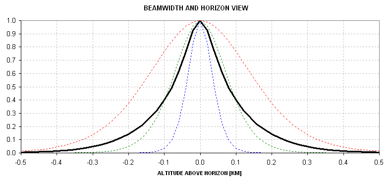
 Figure 5. The MTP/DC8 uses 3 channels, with beamwidths of ~7.7 degrees FWHM, and when flying at 11.4 km the applicable ranges of 2.5, 1.3 and 0.6 km correspond to altitude source functions shown by the dotted traces. The average trace (black) corresponds to using the average brightness temperature for the three channels to establish outside air temperature.

In this figure the average trace (black) should be used as an "averaging kernel" when calculating the layer average brightness temperature for the horizon view used to establish a flight level air temperature. When this is done for the 17-RAOB archive in use for this demonstration the RMS difference between Tw and T is 0.08 K. I note here that this RMS of 0.08 K is artificially low since I'm using RAOBs with poor altitude resolution and invariably over the small altitude region encompassed by the horizontal view source function only one straight line segment of of the RAOB data are sampled and this will produce a zero difference beetween Tw and T when in fact the difference is finite. I will estimate that if the data sampling were closer to true a Tw-T difference of ~0.10 K would be found. That value is used in Fig. 4.

I have chosen to calculate RMS(z) for a DC-8 mission for which I have already performed an exhaustive evaluation of RMS(z) performance. I will use the TOTE/VOTE mission, December, 1995 to February, 1996, which was based mostly in Hawaii. The specific goal of this section is to compare achieved RMS(z) performance with best possible RMS(z) performance for this mission. My purpose is to determine how closely achieved performance approaches best possible performance.

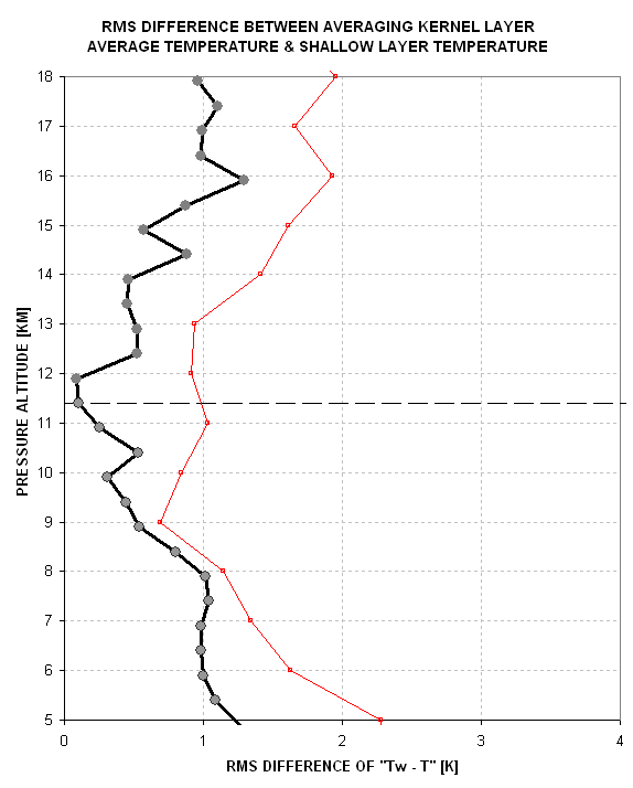
 Figure 6. Measured RMS(z) performance (red) for TOTE/VOTE DC-8 mission, 1992 (details in text), compared with predicted "best possible" (black, same as shown in Fig. 4).

In this figure the measured performance is obtained by comparing retrieved air temperature profiles with nearby RAOBs, described at TOTE/VOTE calibration and RMS Performance Evaluation.

Note the expected behavior of measured performance being worse than "best possible" performace at all altitudes. The difference between these two profiles indicates the presence of an imperfect calibration and/or retrieval algorithm. This difference profile is shown in the next figure.

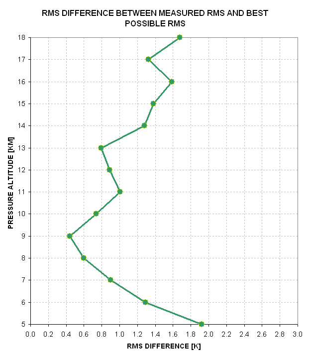
 Figure 7.  Residual uncertainty in retrieved profiles due to calibration errors and retrieval procedure shortcomings.

This figure shows that the retrieved temperature profiles for this mission had an accuracy that was limited by either systematic calibration errors or retrieval algorithm shortcomings, or both, and that these two shortcomings contributed ~1.0 K for the altitude region 7 to 13 km, and less than 2.0 K from 5 to 18 km. The "residual uncertainty" profile in this figure represents how much improvement could theorettically be achieved by performing better calibrations and/or better retrieval algorithms. The goal for any MTP mission is to reduce the residual uncertainty to as close to zero as possible, for all altitudes.

Clever Retrieval Algorithms

It is possible for the "residual uncertainty" profile to be better than zero, or become "imaginary." In other words, it is possible for retrieved T(z) to be better than "best possible." This is because "best possible," as used here, is based on the assumption that averaging kernels are an appropriate way to represent the retrieval process. Dr. M. J. Mahoney has developed clever "iterative statistical retrieval" procedures that can produce T(z) profiles that are better than a classical Backus-Gilbert retrieval procedure. For example, a set of global retrieval coefficients can be used to produce an approximate T(z) profile, and this can be used to select which "profile category" has been encountered, and another retrieval *using the same observables) can be performed using a set of retrieval coefficients calculated (before the mission, for example) based on RAOB T(z) profiles that belong to that "profile category." This process can be repeated as many times as desired, or preferably until some objective criterion of convergence has been met.

Another retrievval scheme that Dr. Mahoney has developed can be employed a day after the flight in question, when RAOBs from along the flight track are available for the time of the flight over those RAOB sites. For example, consider a specific time in a flight that passed near RAOB sites. The time of interest may correspond to part way between sites, and part way from one RAOB sampling time and the next one. A spatial and temporal interpolation can be performed to arrive at a RAOB-suggested profile. This profile can be used as a a template for a search through a large data base of RAOBs to produce a list of actual RAOBs that resembled the template. Ideally, more than 100 such RAOBs would be found. This set of RAOBs can then be used to calculate a set of retrieval coefficients for use with the observables that led to their selection. Amazinlgy good performance can be achieved using this technique. The averaging kernels associated with this retrieval coefficient set would be a misleading guide to expected accuracy, due to the the fact that extra information was used to generate the coeffficients and this information is not explicitly contained in the coefficients. Of course, any benefits from this retrieval algorithm require that calibration errors are small. The only benefit that can be achieved should be thought of as a means for narrowing the altitude thickness of the averaging kernel (that is not reflected by the thickness of the averaging kernel associated with the retrieval coefficients).

It remains to be demonstrated whether a performance that is better than "best possible" can be achieved in practice. This can be a future project for MTP researchers.

This site opened:  November 13, 2004.  Last Update:  November 22, 2004